Modelling COVID-19 in South Africa at a Provincial Level
2021-07-26
MODEL HAS BEEN UPDATED SIGNIFICANTLY FOLLOWING EMERGENCE OF DELTA VARIANT AND FURTHER REVIEW IS PENDING
1 Introduction
This paper documents a model of the COVID-19 epidemic in South Africa. Mobility data is used to model the reproduction number of the COVID-19 epidemic over time using a Bayesian hierarchical model. This is achieved by adapting the work by Imperial College London researchers [1] for South Africa. Authors from Imperial College London have built similar models for Brazil [2] and the United States [3]. In this case the model is calibrated to excess deaths [4] and not case counts or reported COVID-19 deaths.
The model uses mobility movement indexes by province produced by Google [5]. Furthermore the model includes a fixed effect for interventions introduced at the start of level 4 lockdown.
The model and report are automatically generated on a regular basis using R [6]. This version contains data available on 17 July 2021.
An online, regularly updated version of this report is available here.
2 Updates
As this paper is updated over time this section will summarise significant changes. The code producing this paper is tracked using git. The git commit hash for this project at the time of generating this paper was e802ad83e4c6ac385891b380e7289a0e83c9a511 and this change was made on 2021-07-26.
The changes summarised below excludes the weekly updates to excess deaths.
2020-05-31
- Document is made available online (pending review).
2020-06-01
- Added backtesting.
2020-06-04
- Incorporated feedback from reviewer 1.
2020-06-08
- Incorporated feedback from reviewer 2 and 3.
- Added a projection for South Africa (based on sum of the provinces).
- Created a CSV with the daily projections. See the projection section for details.
- Added an updates section to track changes to this model.
2020-06-09
- Incorporate feedback from reviewer 4.
- Remove the under review designation. As at this date the model has feedback from 4 reviewers and also comments from others. The author will continue to update this model and seek review as needed.
- Due to mobility increasing from level 3, additional projection scenarios have been introduced involving decreased mobility (back to level 4 levels).
- Numerous updates on plots including some residual plots.
2020-06-10
- Remove parks index from average mobility index in line with [7]. Will drop residential index soon too.
2020-06-20
- Update IFRs for HIV. Possibly need further increases based on research coming out in near future.
- Remove residential mobility, such that there is only one mobility parameter left.
2020-06-22
- Add parameter for fixed effects correlated with the start of level 4 lockdown aimed at capturing the effect of mask wearing and workplace screening.
2020-07-04
- Updated standard deviation of prior for \(\beta\) to reflect [8]. This allows for a greater impact of mask wearing on \(R_{t,m}\).
- Update on prior assumption for provincial effect of interventions implemented at start of level 4 lockdown.
2020-07-07
- Major changes to allow for excess deaths exceeding reported COVID-19 deaths.
- Expanded calibration graphs for more provinces.
2020-07-16
- Increase uncertainty around completeness of reporting factors.
2020-07-26
- Remove 14-day backtesting to reduce total run time.
- Further update to excess deaths calculation to give reporting data an additional week of run-off.
2020-08-19
- Incorporate autoregressive term in modelling of \(R_{t,m}\) to improve fit using approach in [9].
- Switch to using excess deaths as the outcome to be modelled rather than reported deaths.
- Remove backtesting to improve run time. Will add it back once model is stable.
2020-09-05
- Update percentage of excess deaths (\(\psi\)) distribution to narrow the variance.
2020-11-24
- Fixed an issue with how excess deaths were processed.
2020-11-28
- Update infection fatality rates to those from [10]. These are slightly lower than those from [11], [12] and [13].
- Add worst case projection.
- Add projection output for 31 March 2021.
2020-12-14
- Show correct estimates for \(R_{0,m}\). Previous the initial values of \(R_{t,m}\) were shown which in theory would be correct, except that for some provinces the projections only start after lockdown and hence the initial values of \(R_{t,m}\) is well below \(R_{0,m}\).
- Show estimates of deaths to date.
2021-01-01
- Corrected parameter estimate plots. These charts were incorrectly adding country wide effects and provincial effects.
2021-01-11
- Add projection to 30 June 2021
2021-01-24
- Align weeks to CDC weeks in step with the source.
2021-04-29
- Update projection dates to 30 June and 30 September 2021.
2021-06-01
- Adjust mobility scenarios.
2021-06-30
- Allow for increased transmission of Beta variant.
- Add the emergence of Delta variant.
- Remove provincial intervention and mobility effects to speed up model.
- Update projection dates to 30 September and 31 December 2021.
- No longer revert AR(2) term to 0 for worst case projection.
- Use a single \(R_{0}\) for all provinces instead of provincial specific \(R_{0,m}\) to simplify the model.
- Update many of the charts to show better effects of the parameters of the model for \(R_{t,m}\). Some of the effects will appear larger and smaller but have not changed meaningfully.
3 Methodology
A detailed description of the methodology and assumptions is provided below below. The key features of the approach employed are summarised here:
- It uses a Bayesian Hierarchical Model to calibrate model parameters based on observed excess death data and prior assumptions.
- Changes in the reproduction number are linked to mobility data [5], the introduction of other non-pharmaceutical interventions (NPIs), as well as an autoregressive term.
- The reproduction number over time is used to model the number of infections occurring over time.
- The model uses population-weighted infection fatality ratios (IFRs) by province with some noise added as well as assumptions about the time it takes to die to model deaths from infections.
- There is a single combined model for all provinces. This model shares information between provinces, but province-specific effects are also allowed.
- The model is fitted such that it uses the prior assumptions about various parameters as well as the excess death data provide an updated parameter distribution and outcome distribution that reflect both the prior assumptions as well as the excess death data.
4 Mobility
4.1 National Mobility Data
The national mobility data from [5] is plotted below. The model uses the indexes at a provincial level but here the national indexes are plotted for convenience. Clear trends are observable:
- Mobility generally reduces before the lockdown on 27 March (except for residential mobility).
- There is an increase in mobility in the days just before the lockdown. In particular the Grocery & Pharmacy and Retail indexes. Perhaps an indication of pre-lockdown “panic buying?”
- Mobility is relatively stable during level 5 lockdown at low levels.
- Mobility increases when level 4 starts.
- Mobility dropped at the start of 2021 and has generally been rising since.
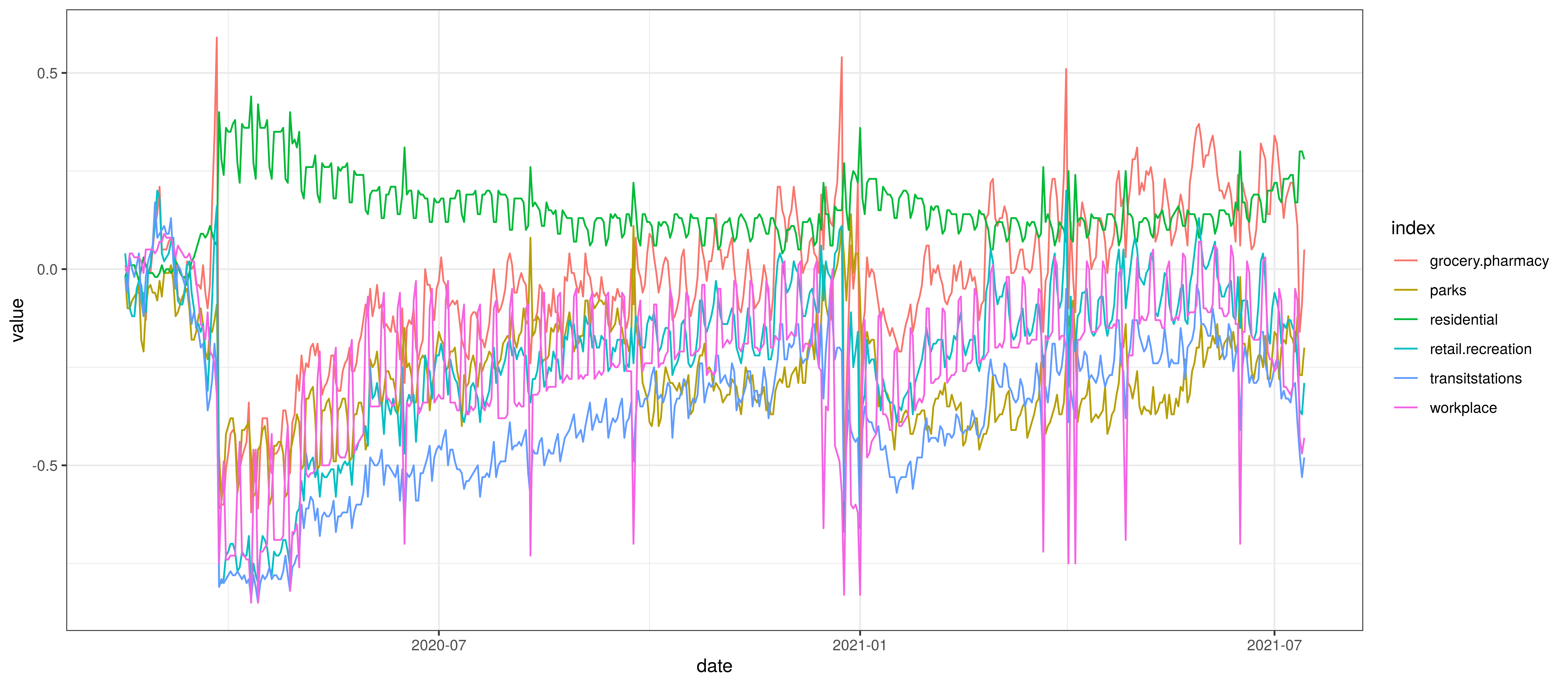
Google Mobility Indexes for South Africa
The chart below summarises the average mobility index used in the model. This is the average of mobility indicators excluding parks and residential. This follows [7].
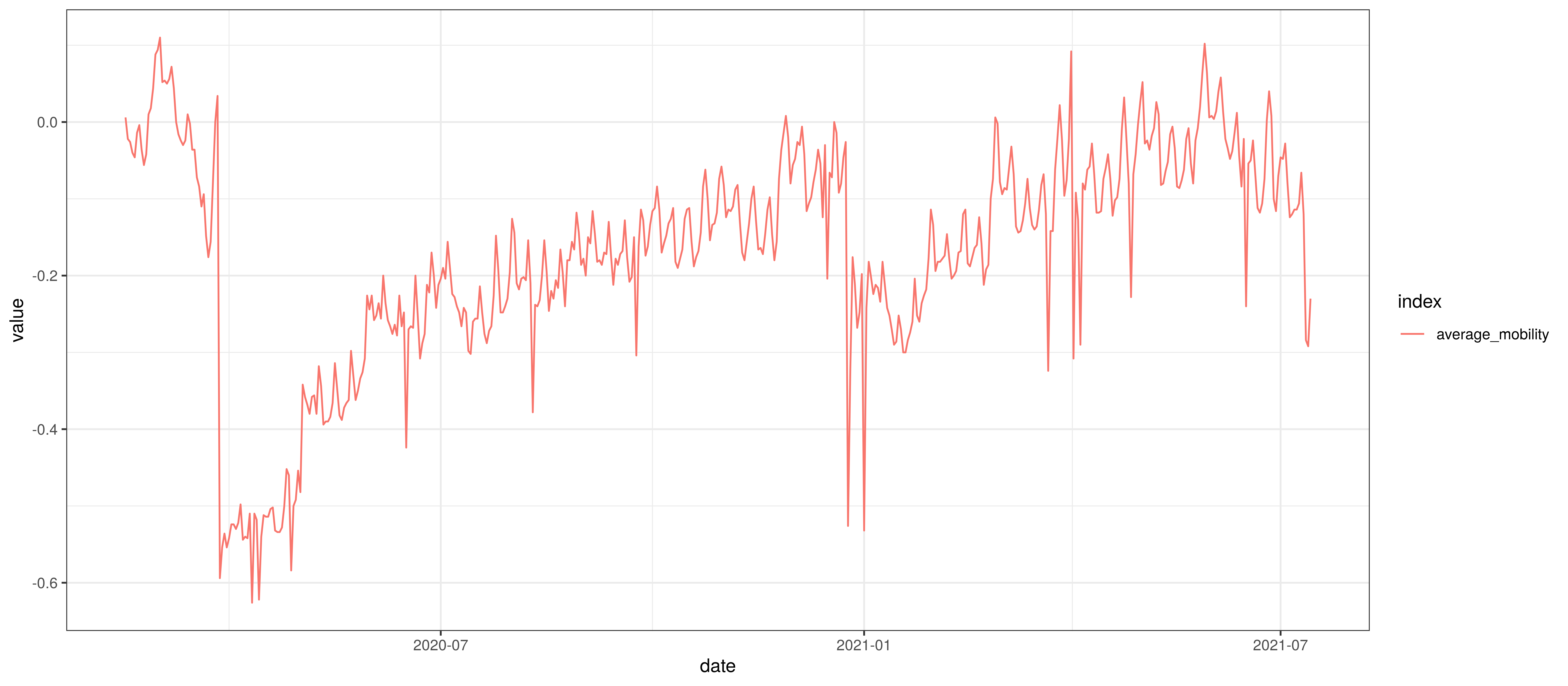
Average Mobility
There are some risks to using the mobility data above as it may be biased to the Android operating system, people with smartphones and people with enough data on their smartphone to share their location.
This bias does not really represent a problem though unless it changes over time because then the model would not be able to produce accurate projections. There is a risk that mobility changes disproportionally between users contributing data to these indexes and those not. It would not seem reasonable to expect a major change in the bias over time (unless the calculation is somehow compromised). Provincial biases may exist, but the model does not allow for provincial-specific mobility effects as none was observed in the fitting of the model.
4.2 Provincial Mobility Data
The average mobility (excluding residential & park indexes) is plotted below for the various provinces. From this plot it seems apparent that Western Cape mobility is generally lower than other provinces.
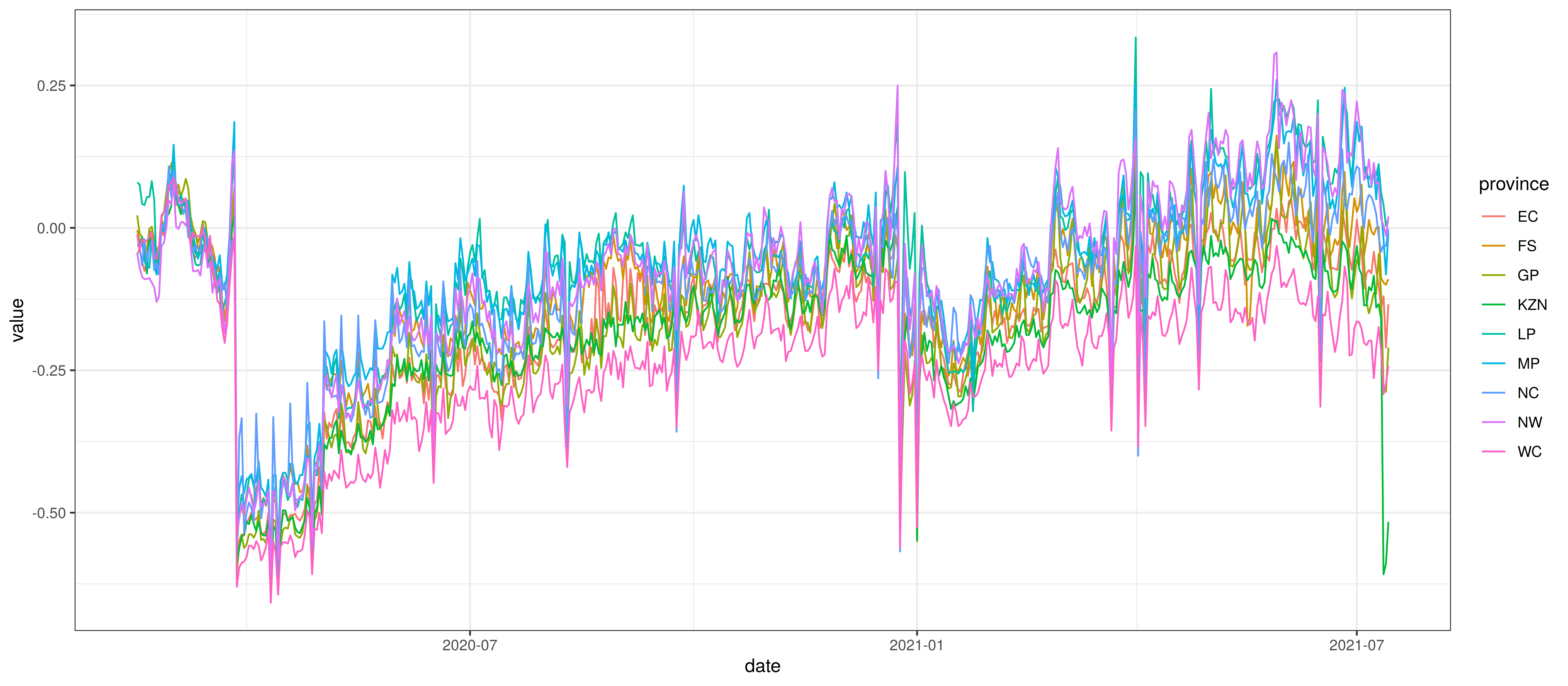
Average Mobility by Province
5 Calibration
The sections below show how well the model is reproducing past excess death data. As the model is fitted to past death data we would want to see how well it is reproducing such data. Each section covers a province.
Various panels are plotted for each province:
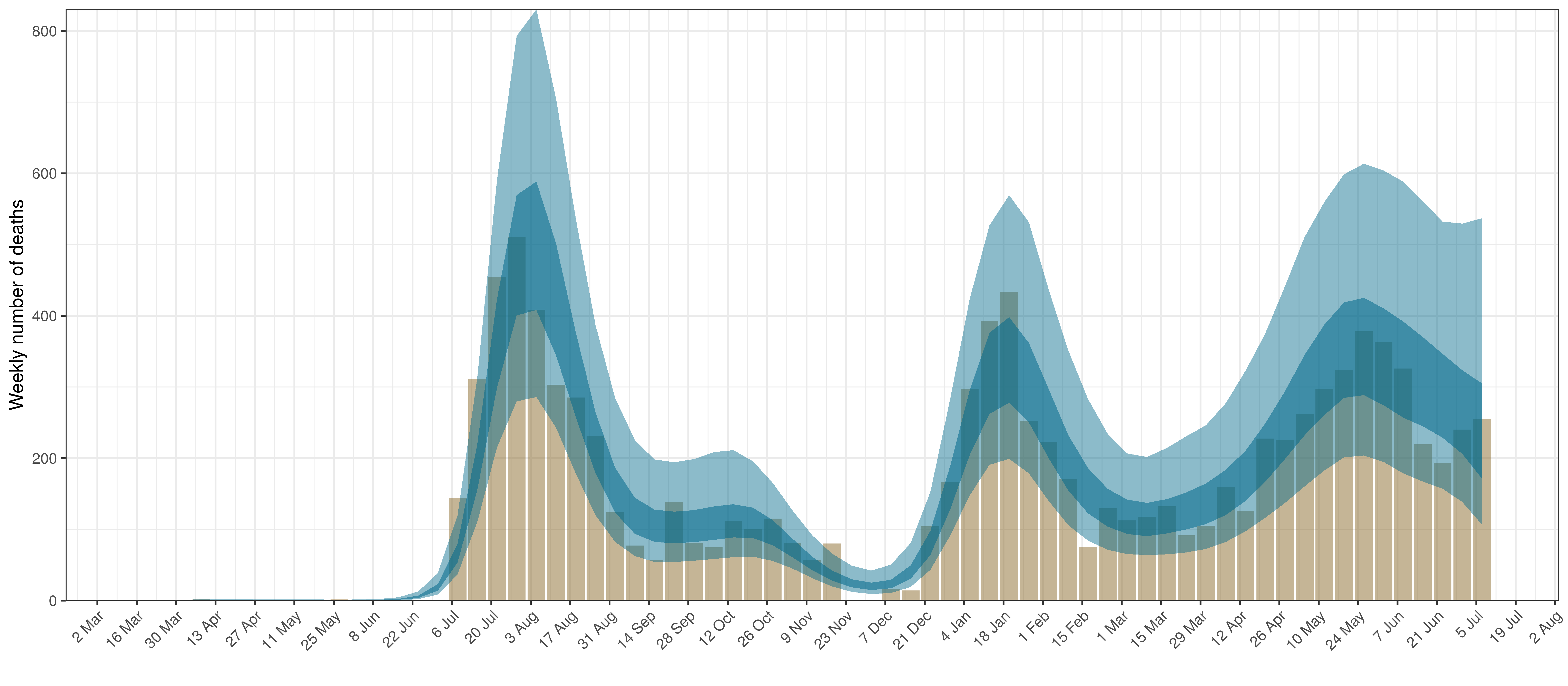
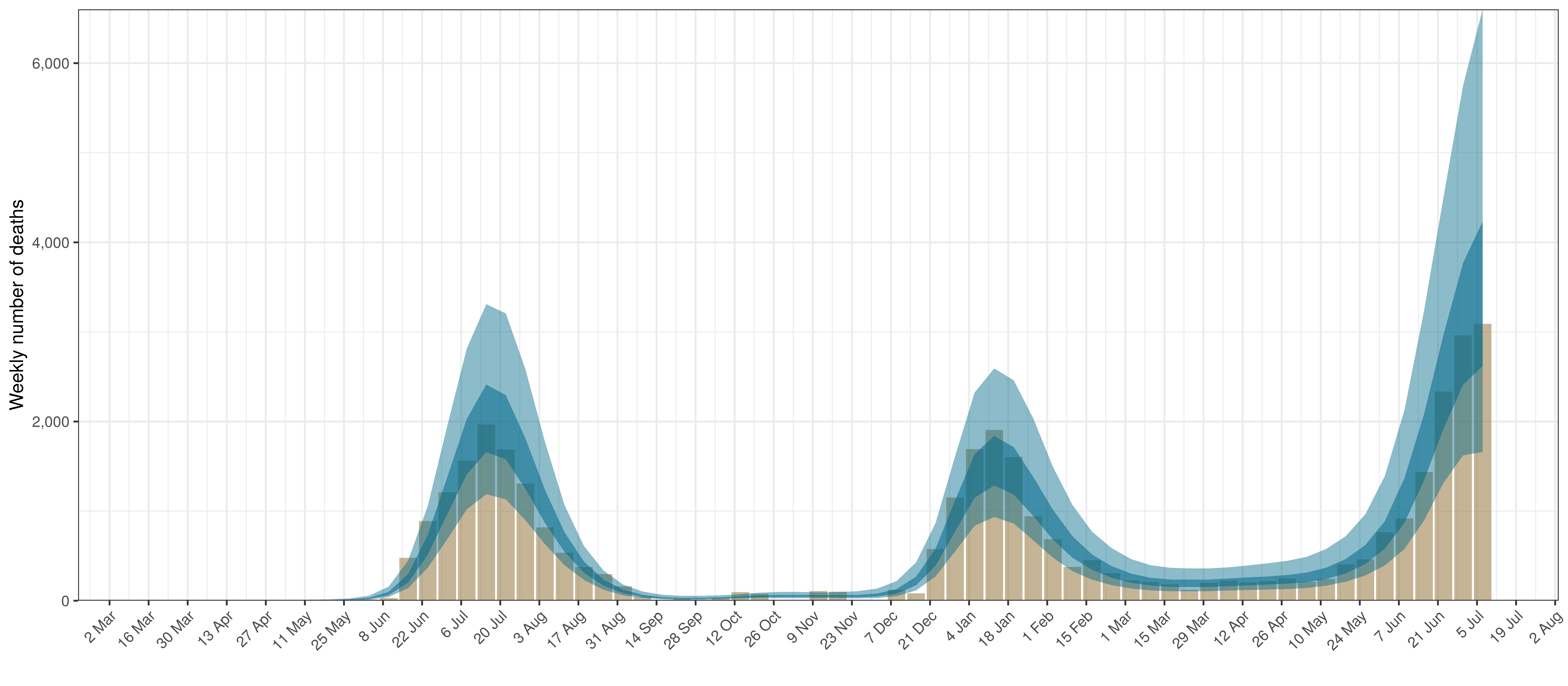
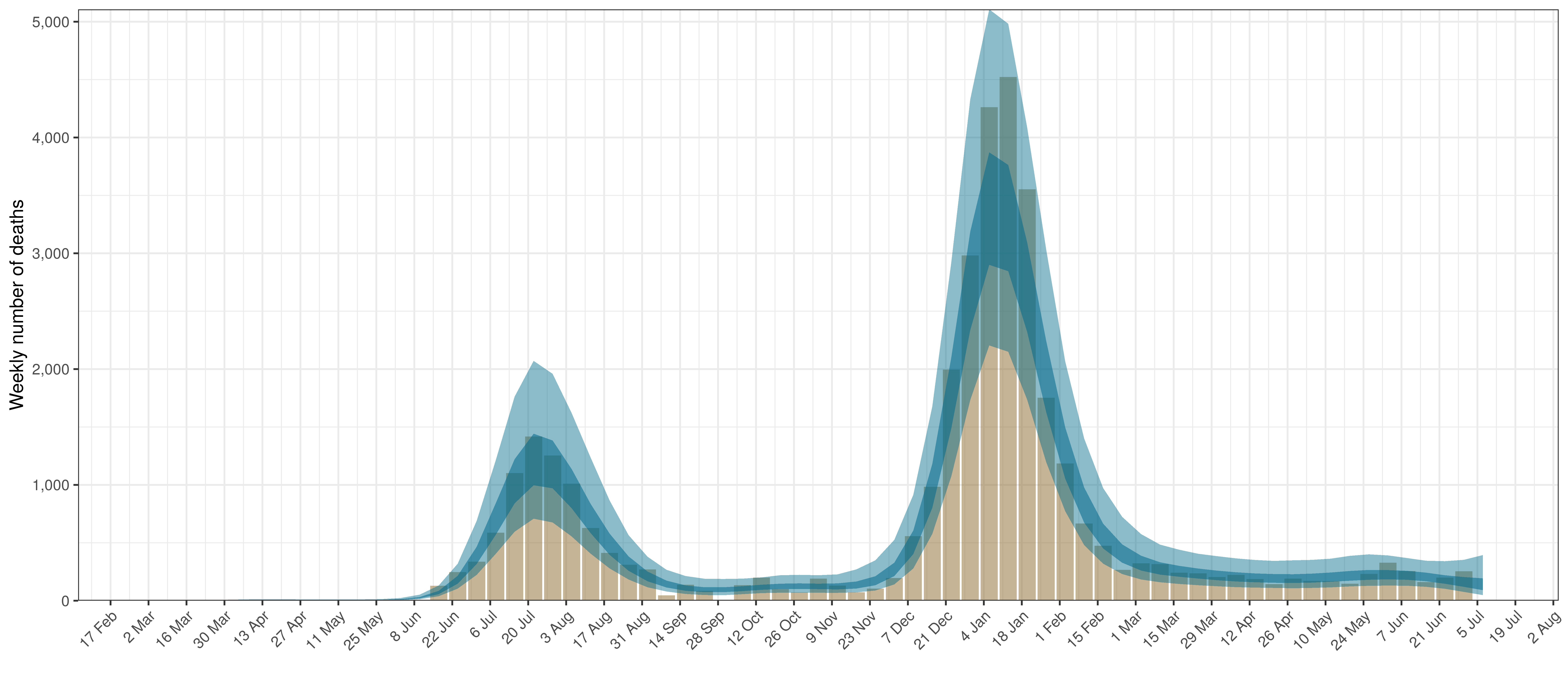
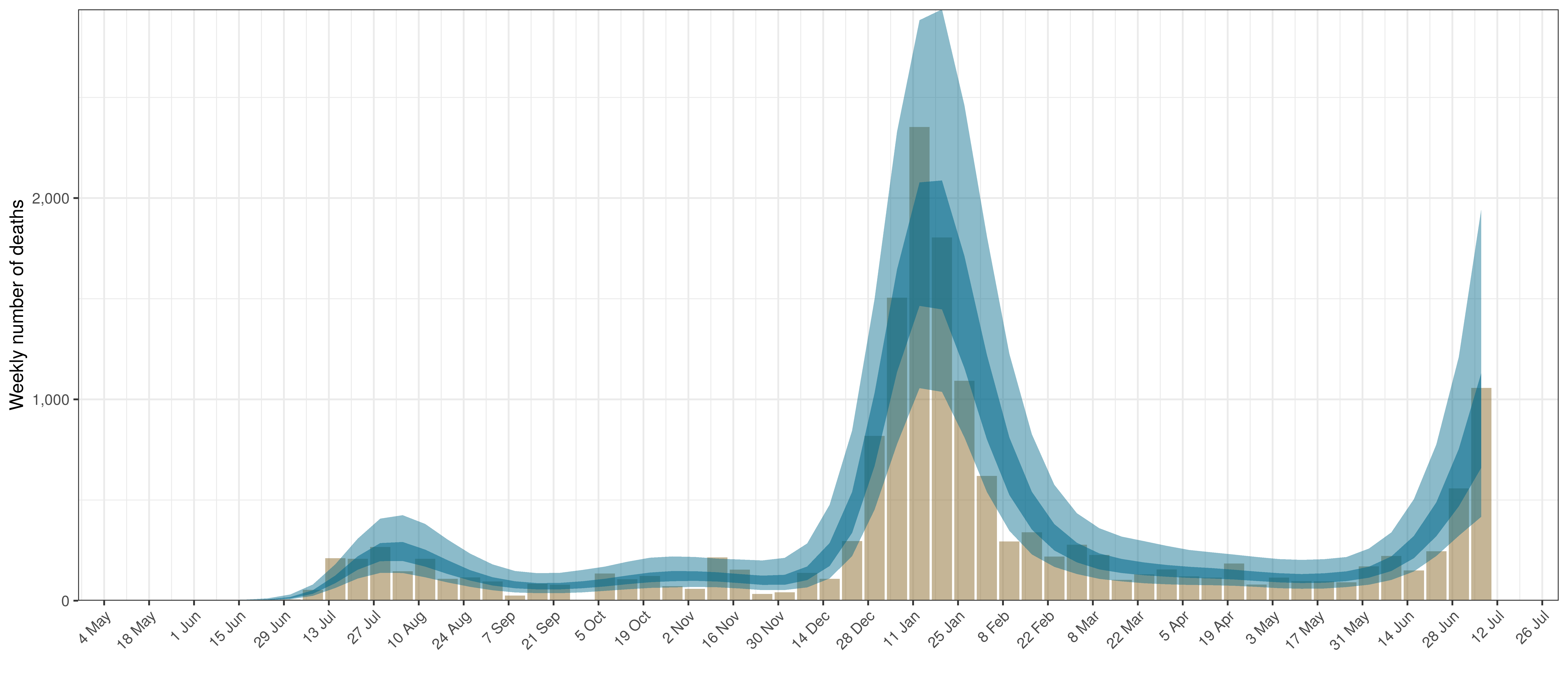
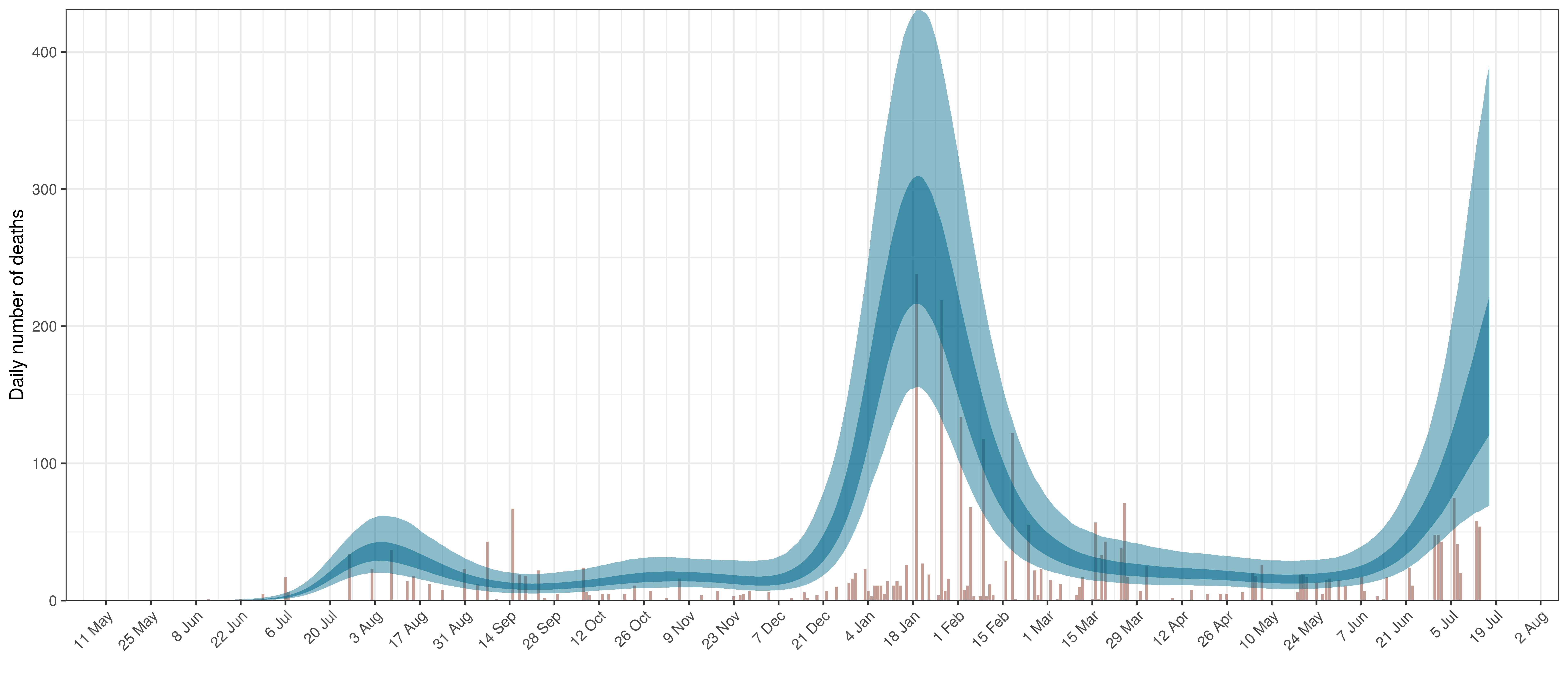
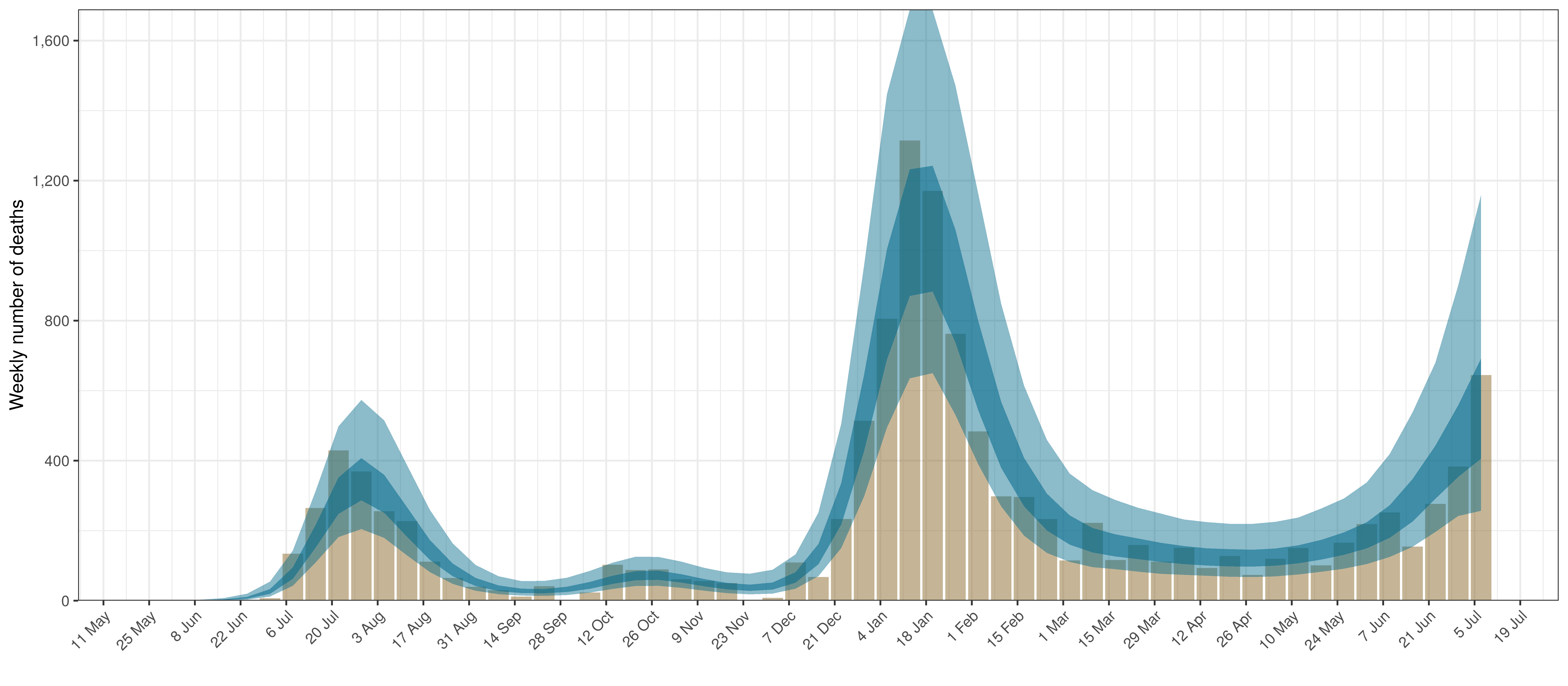
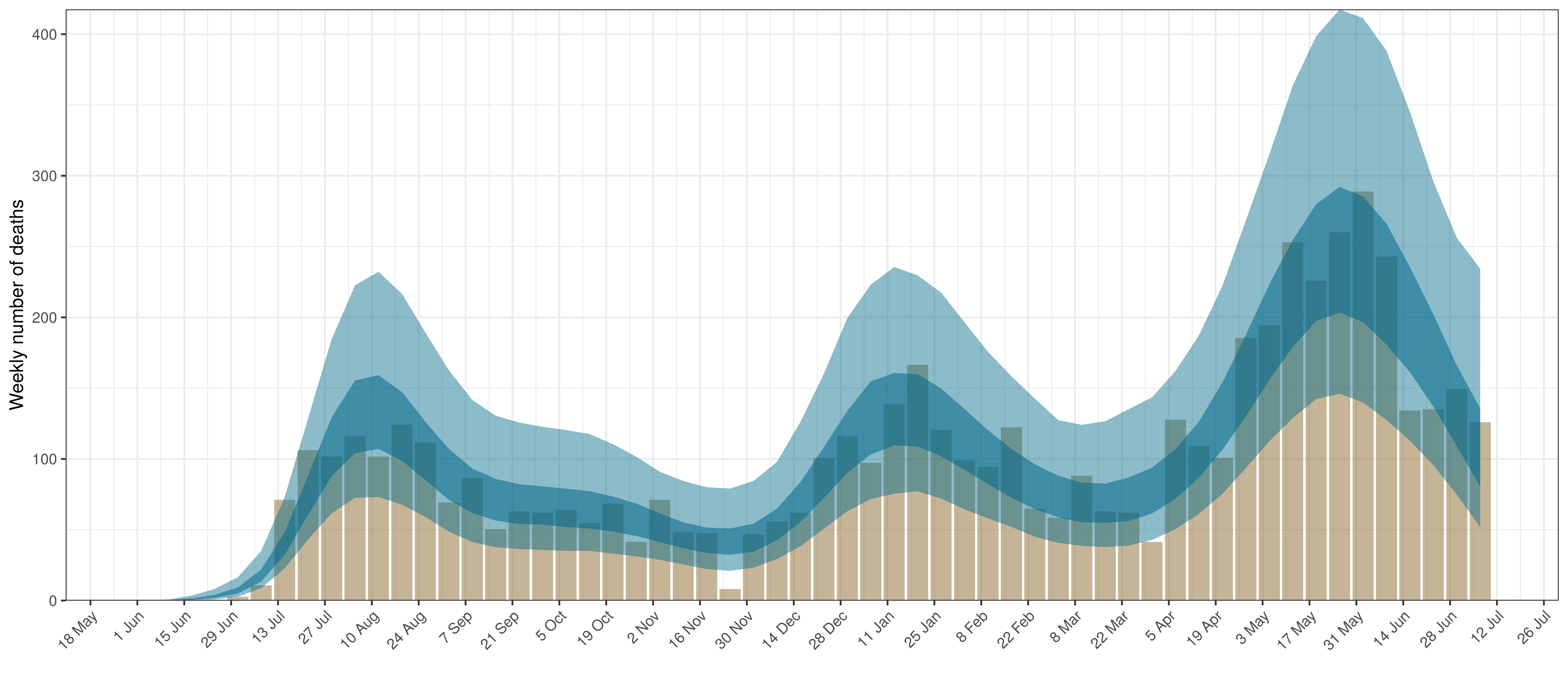
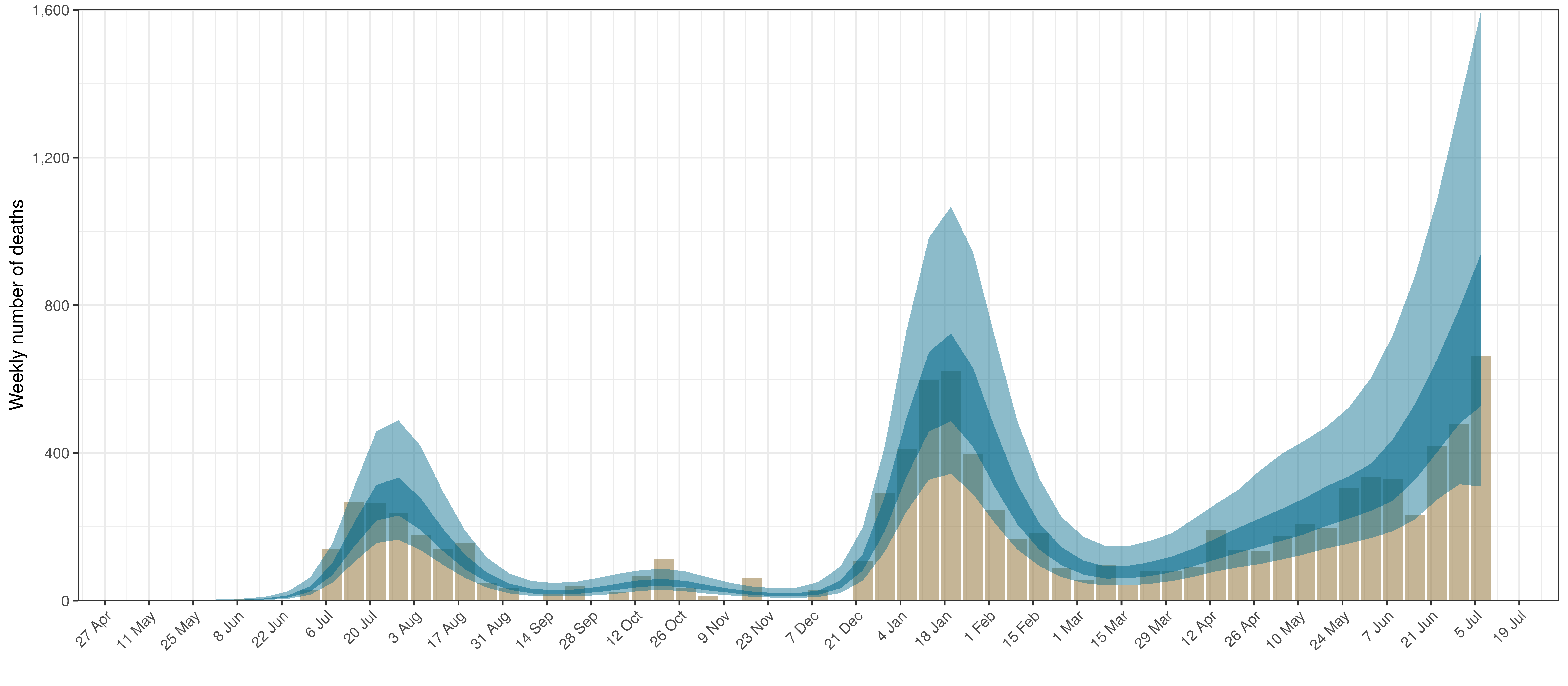
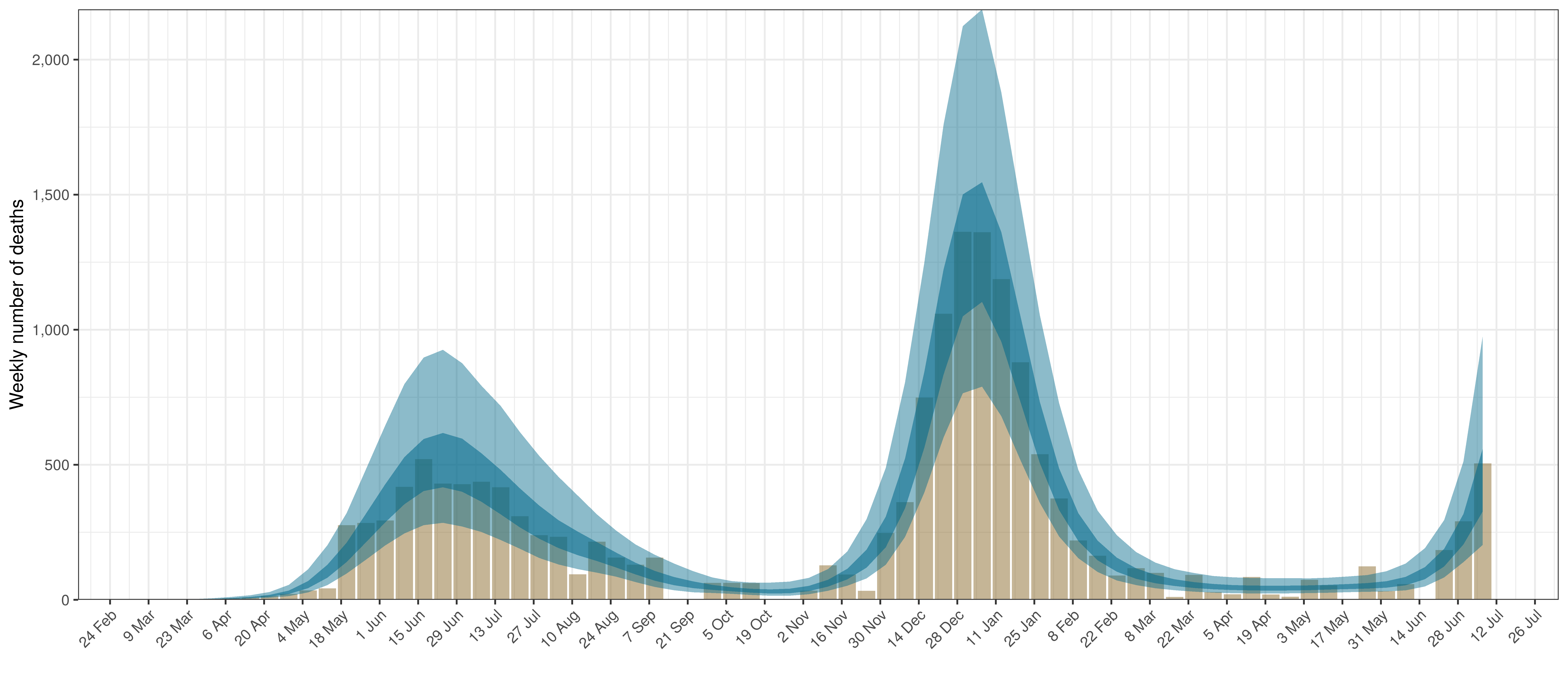
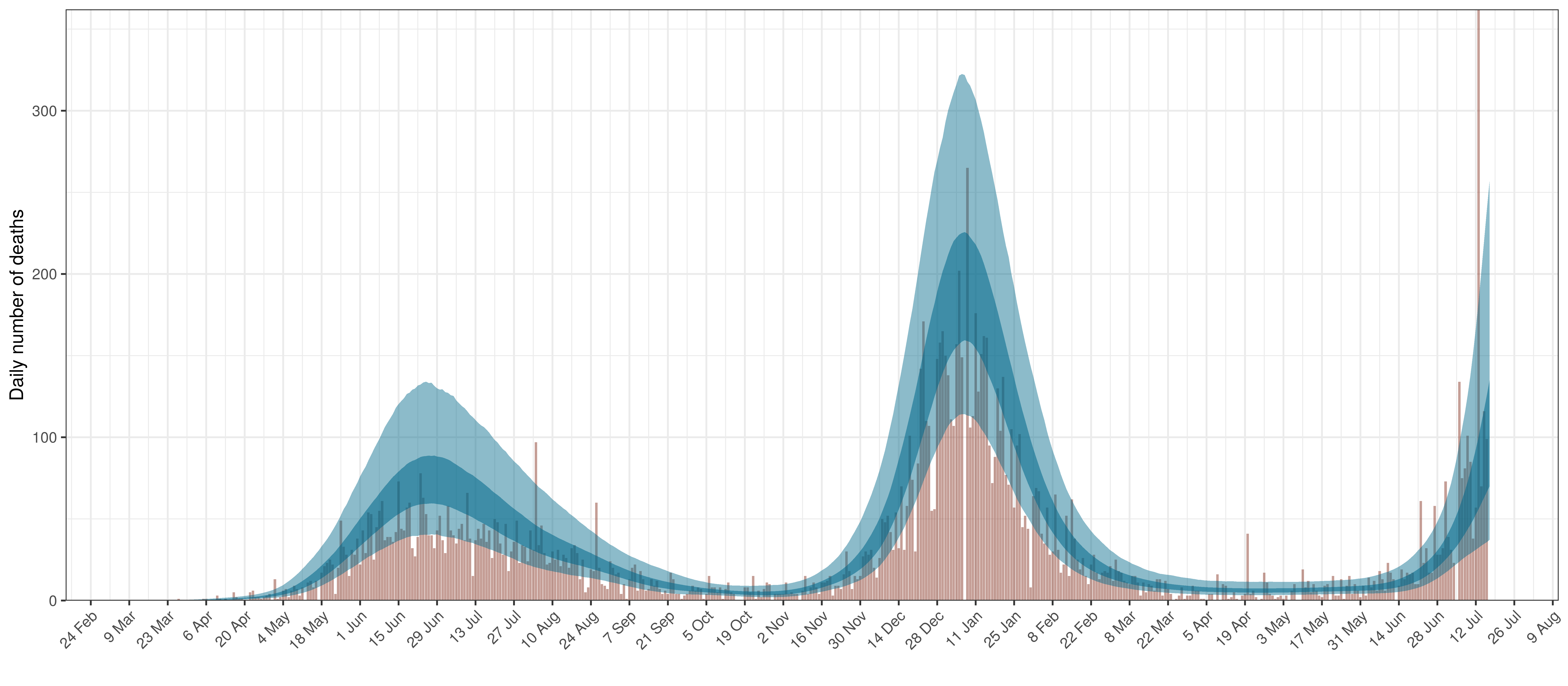
- The first panel shows modelled weekly deaths (blue) and 90% of excess deaths (brown). Bars are plotted at the start of the week (which coincides with [4]). A good model would produce death forecasts such that the actual reported past deaths would appear in the confidence intervals of the prediction.
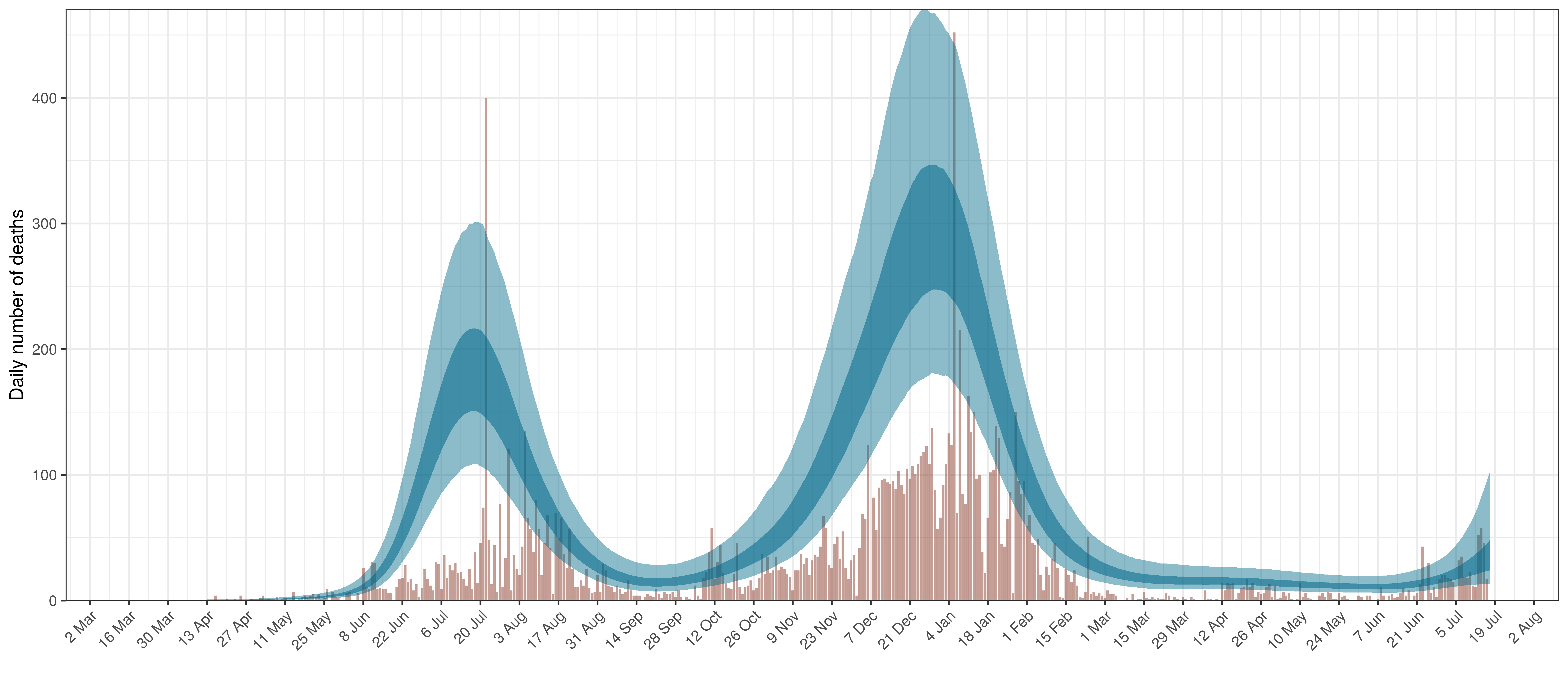
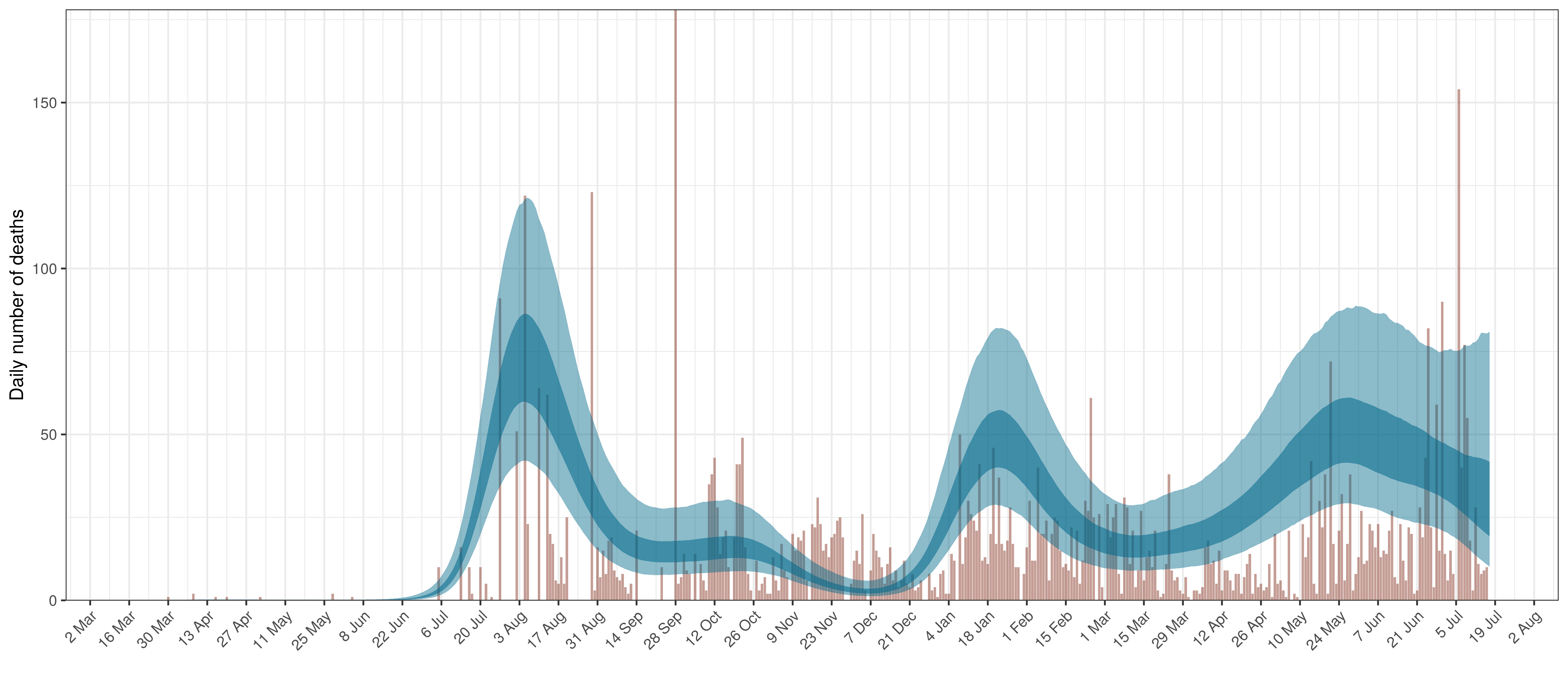
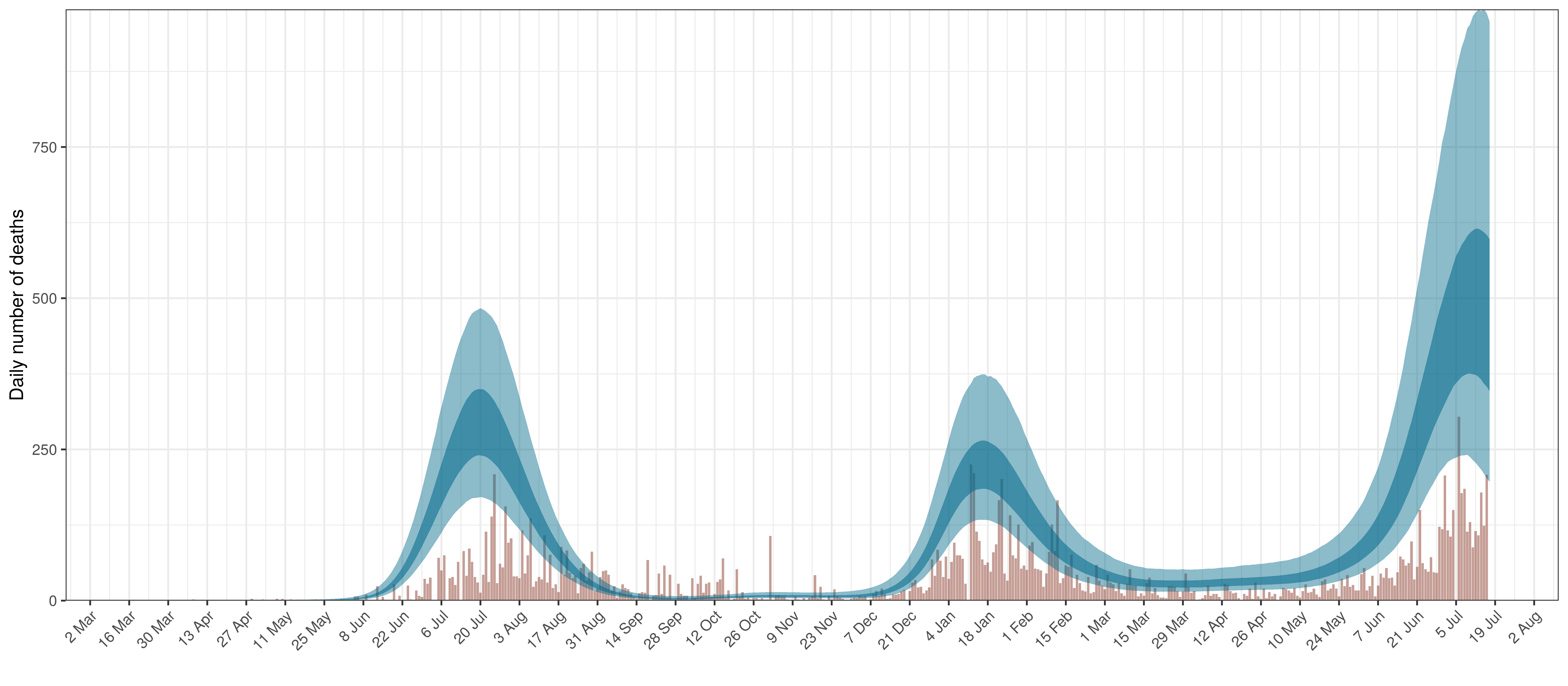
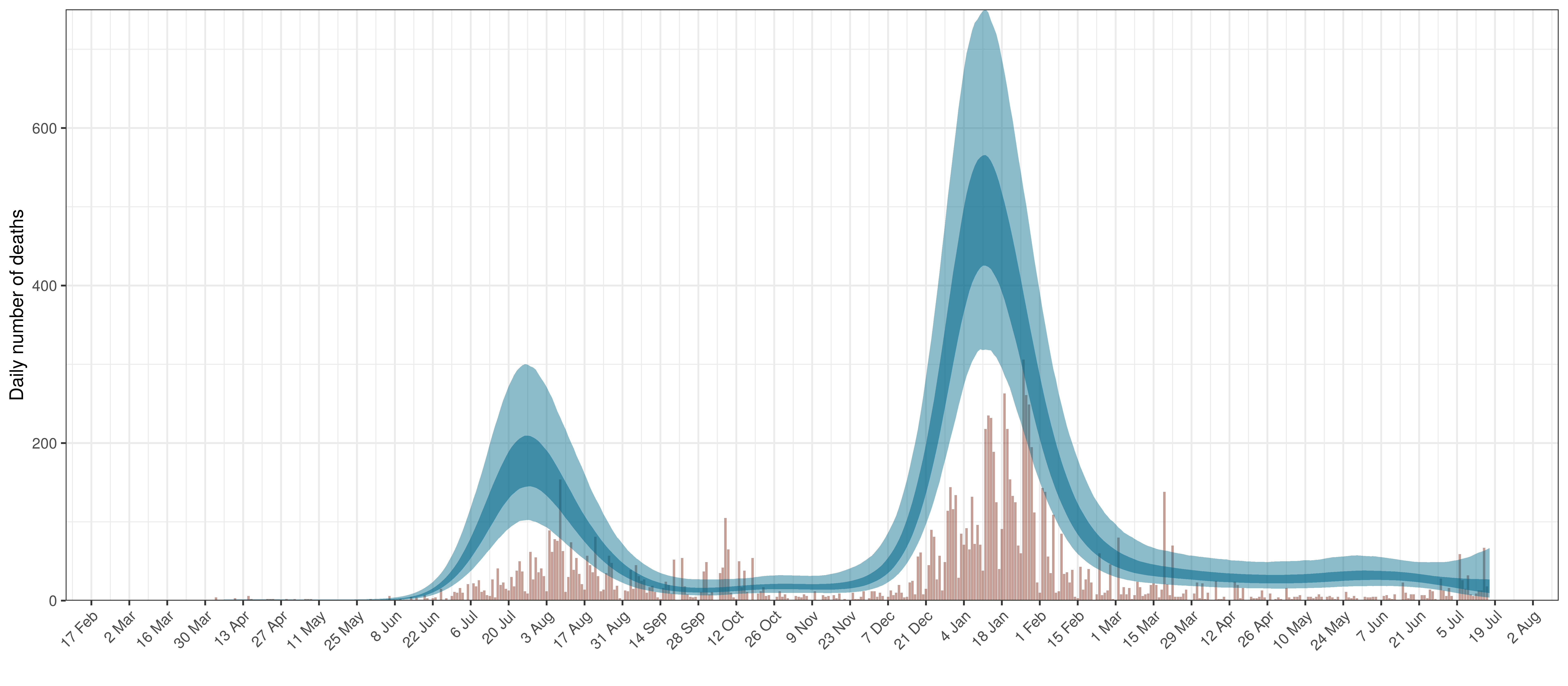
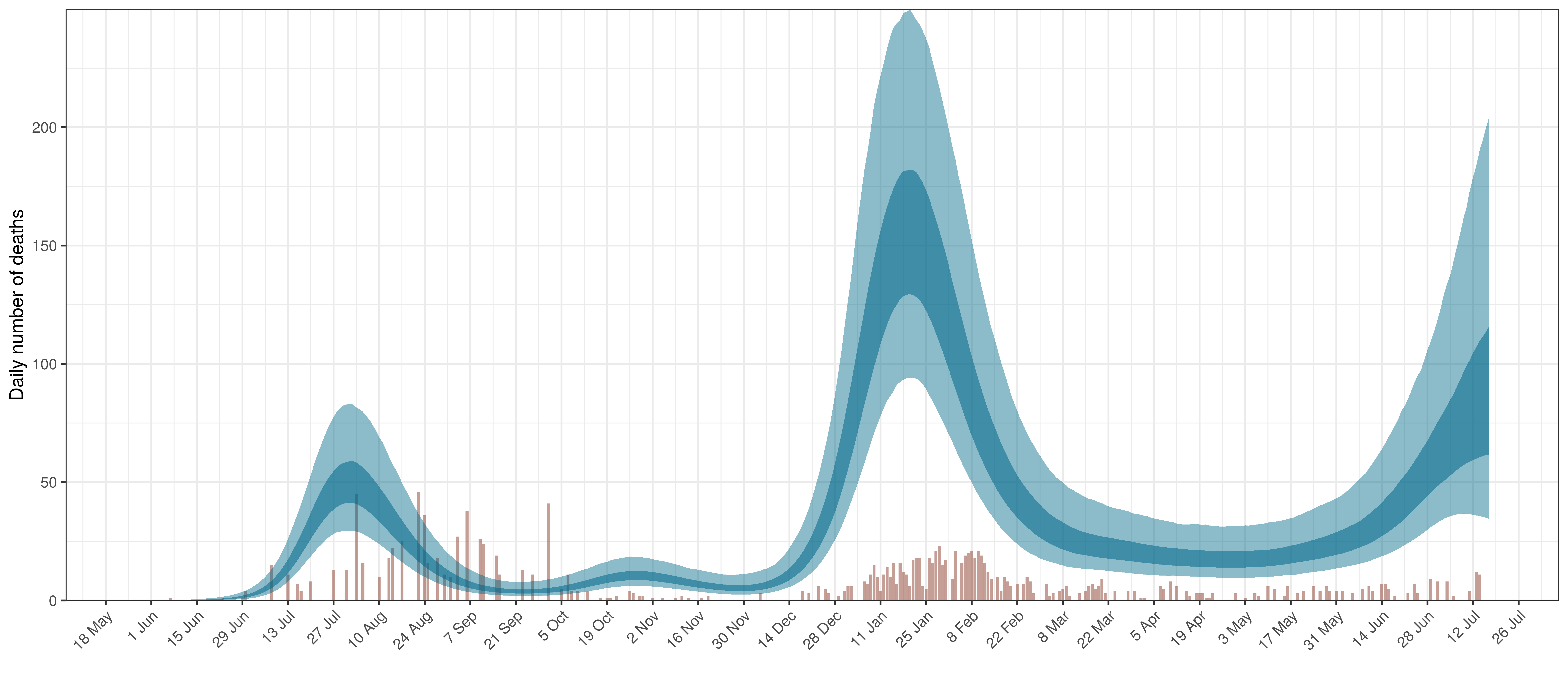
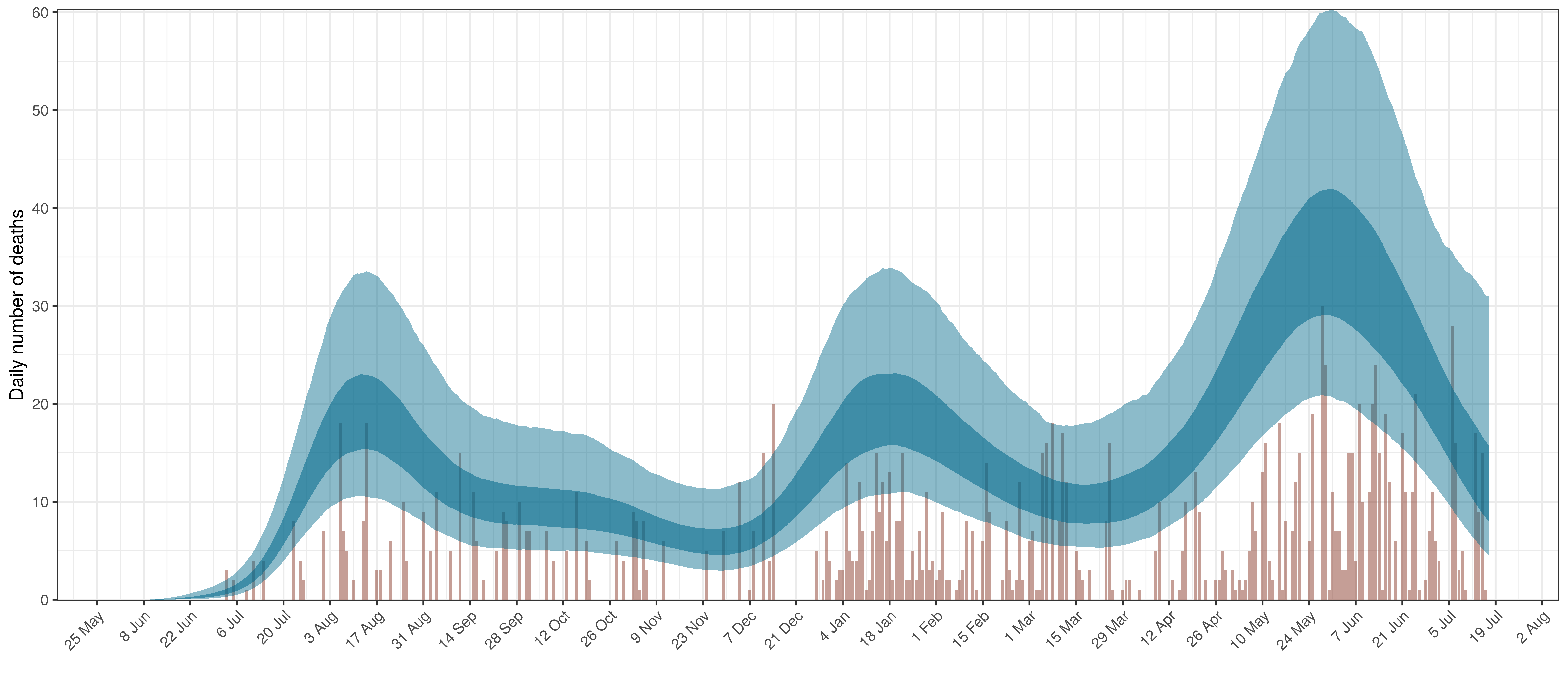
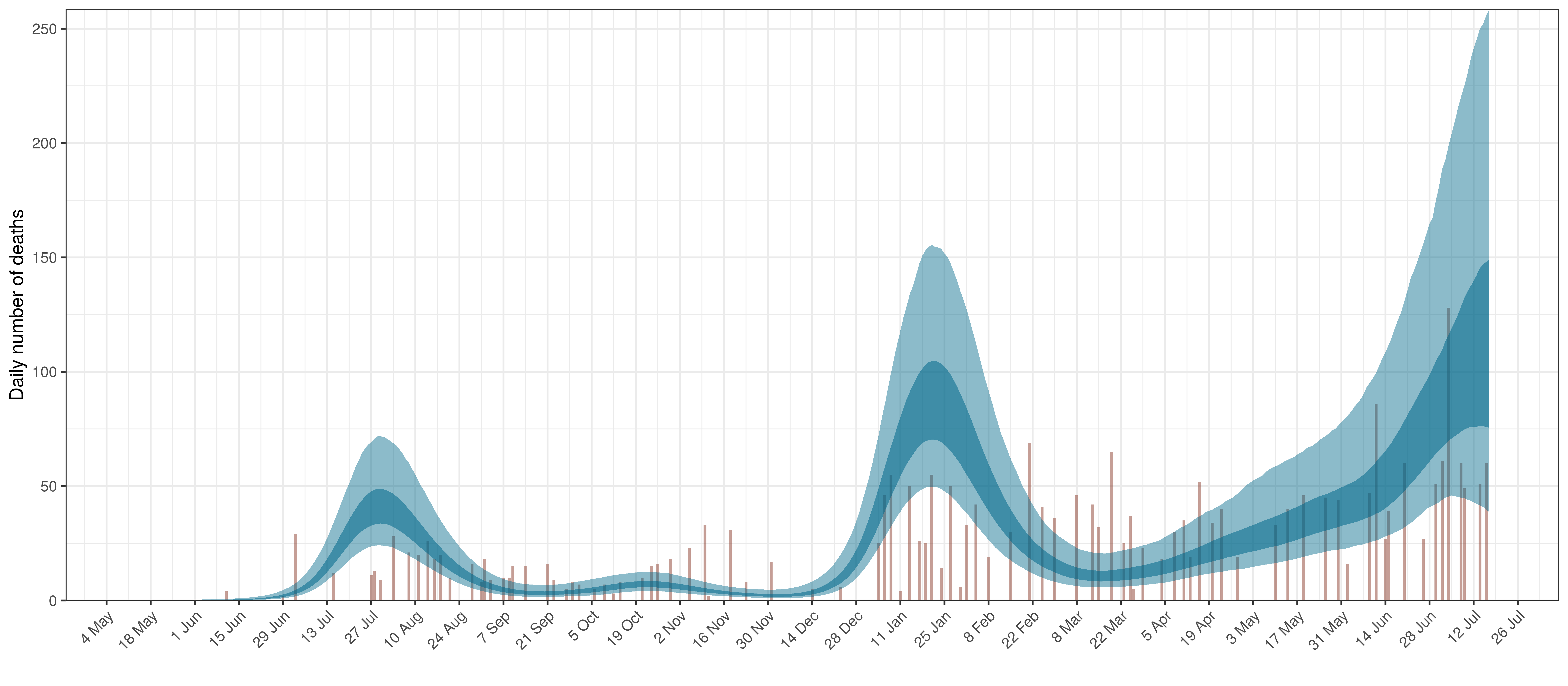
- The second shows the daily count of deaths reported in the province (brown) and the estimated deaths in blue.
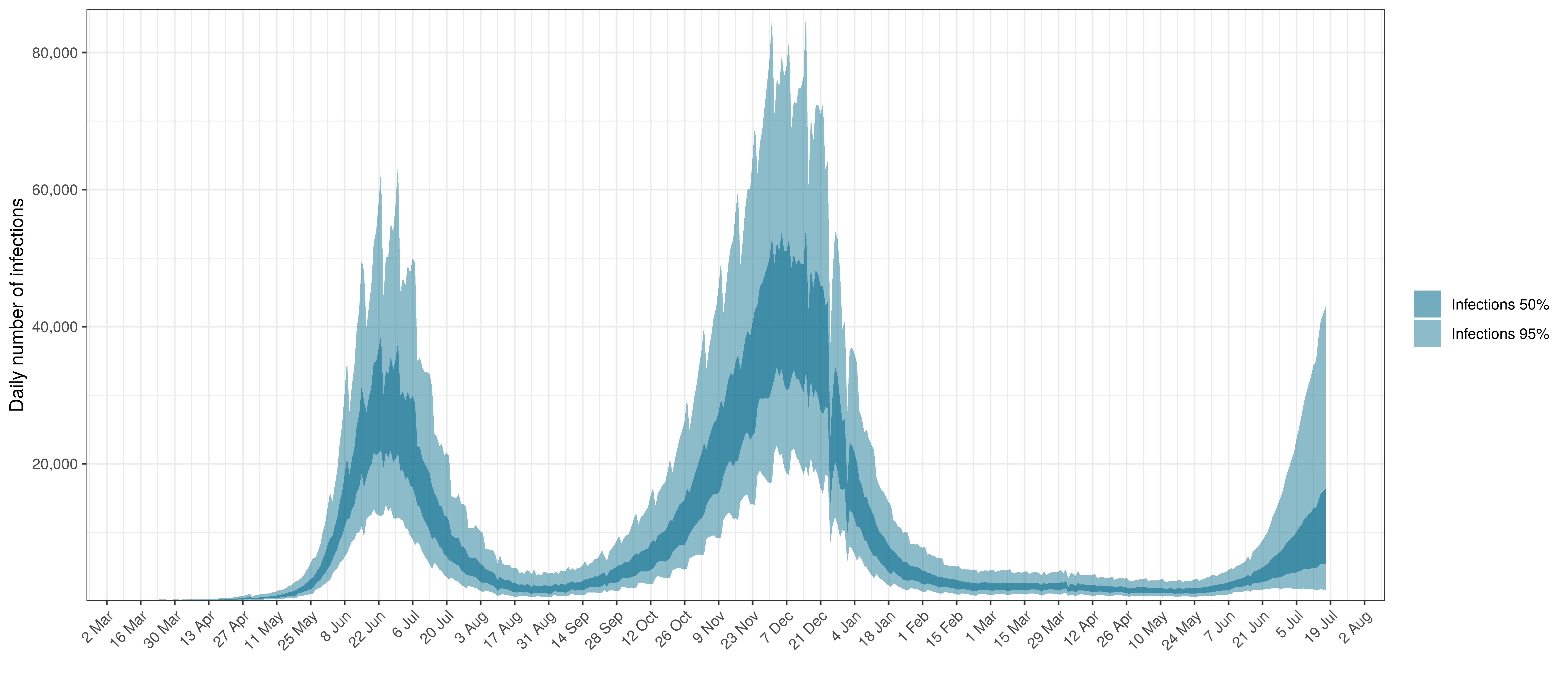
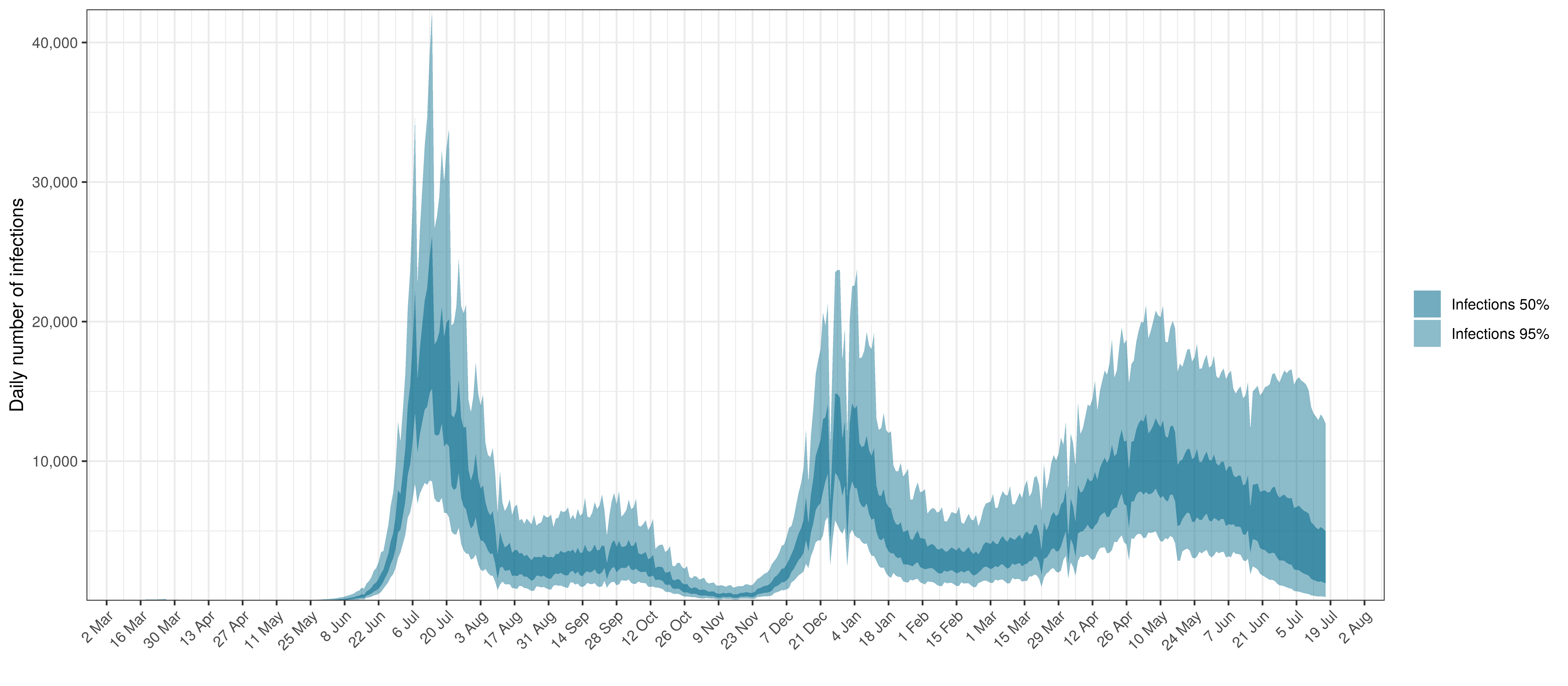
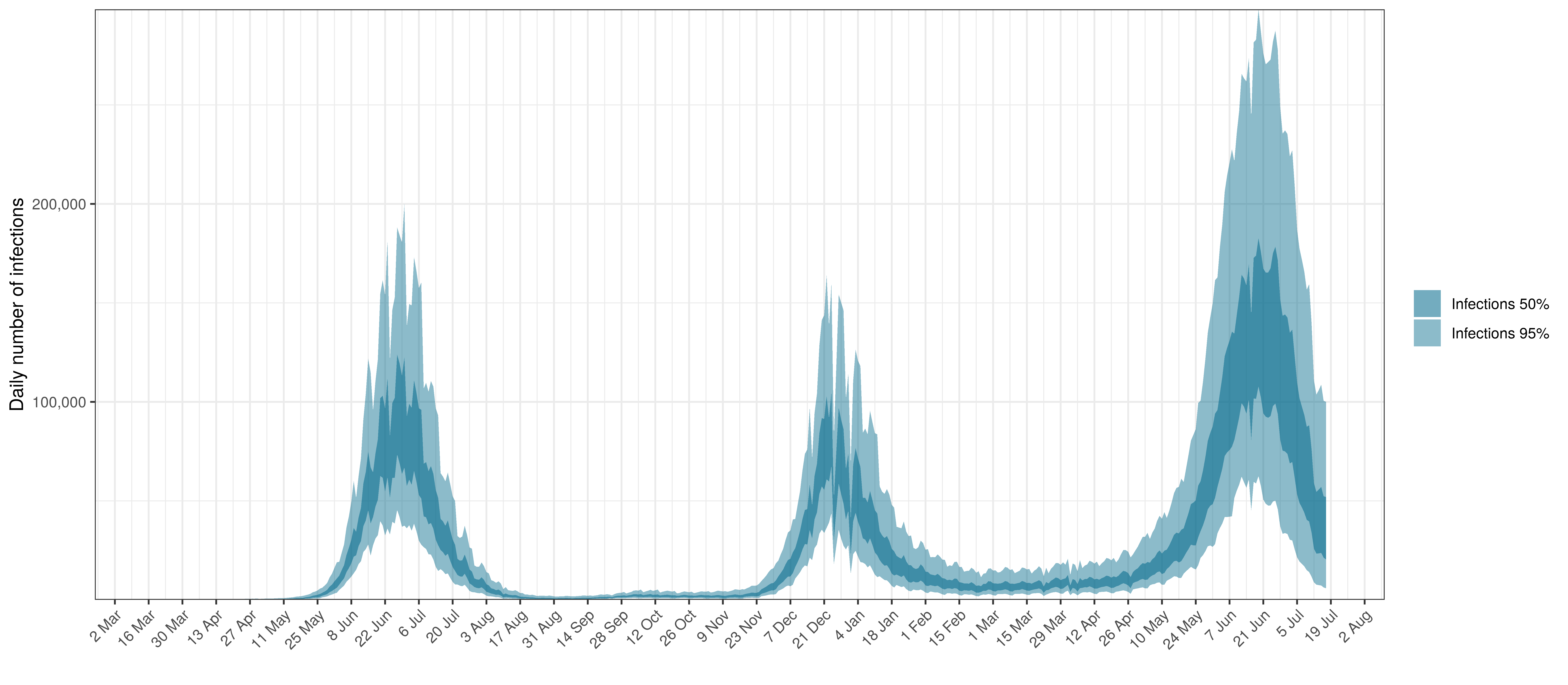
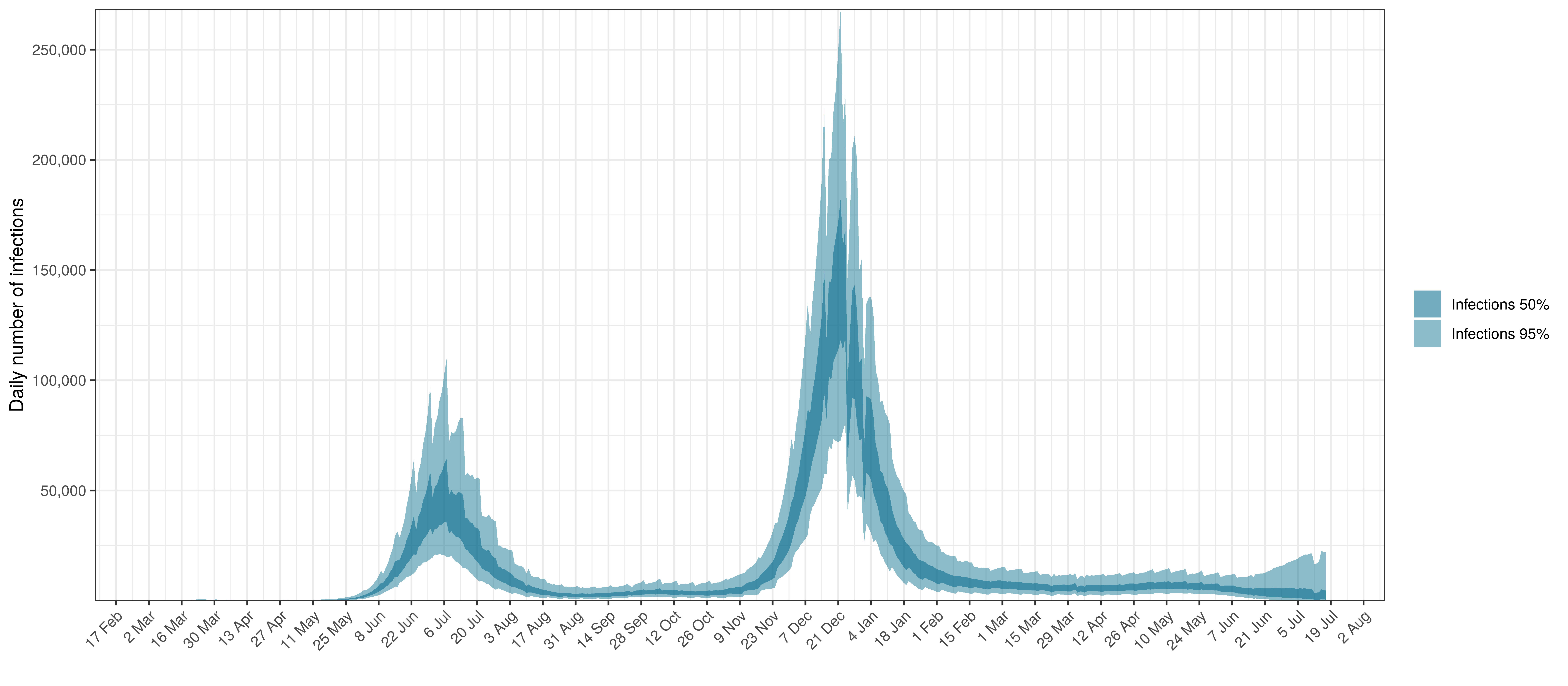
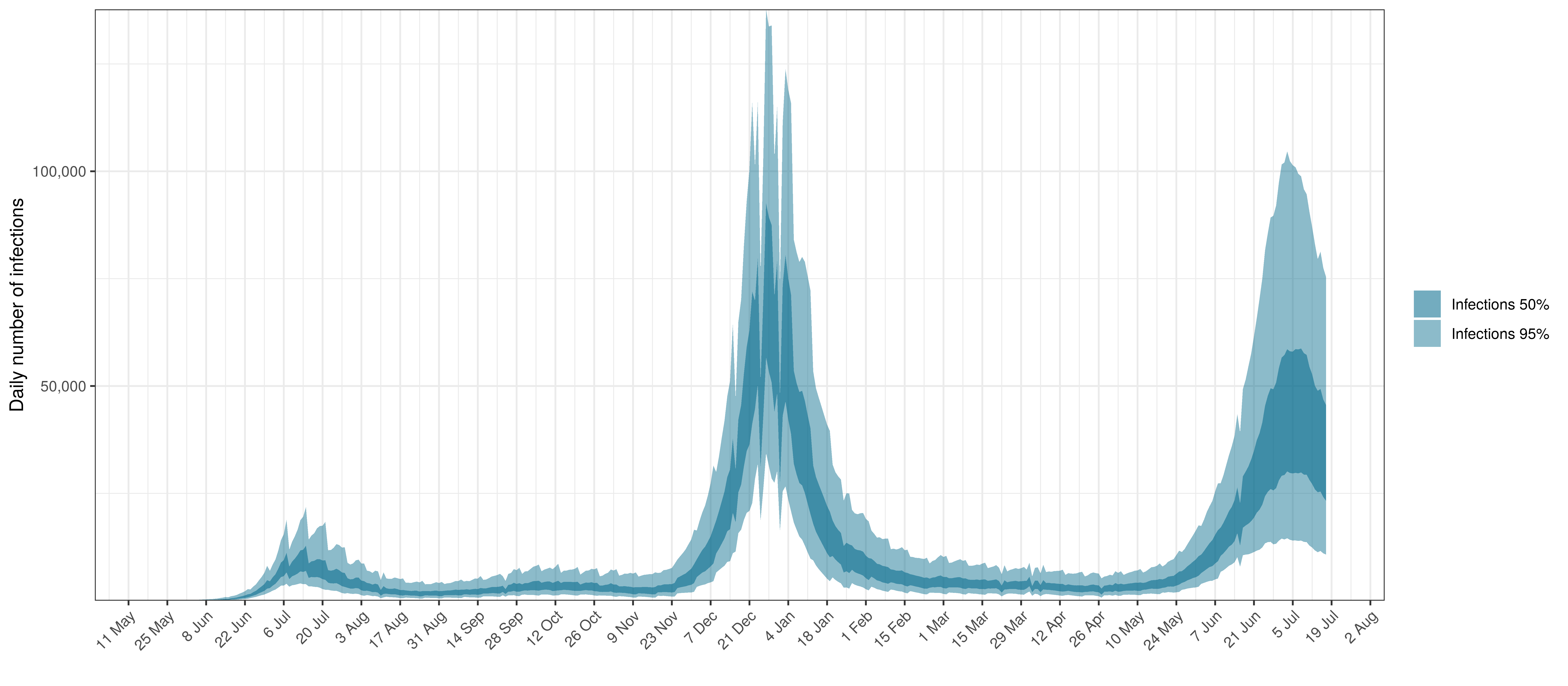
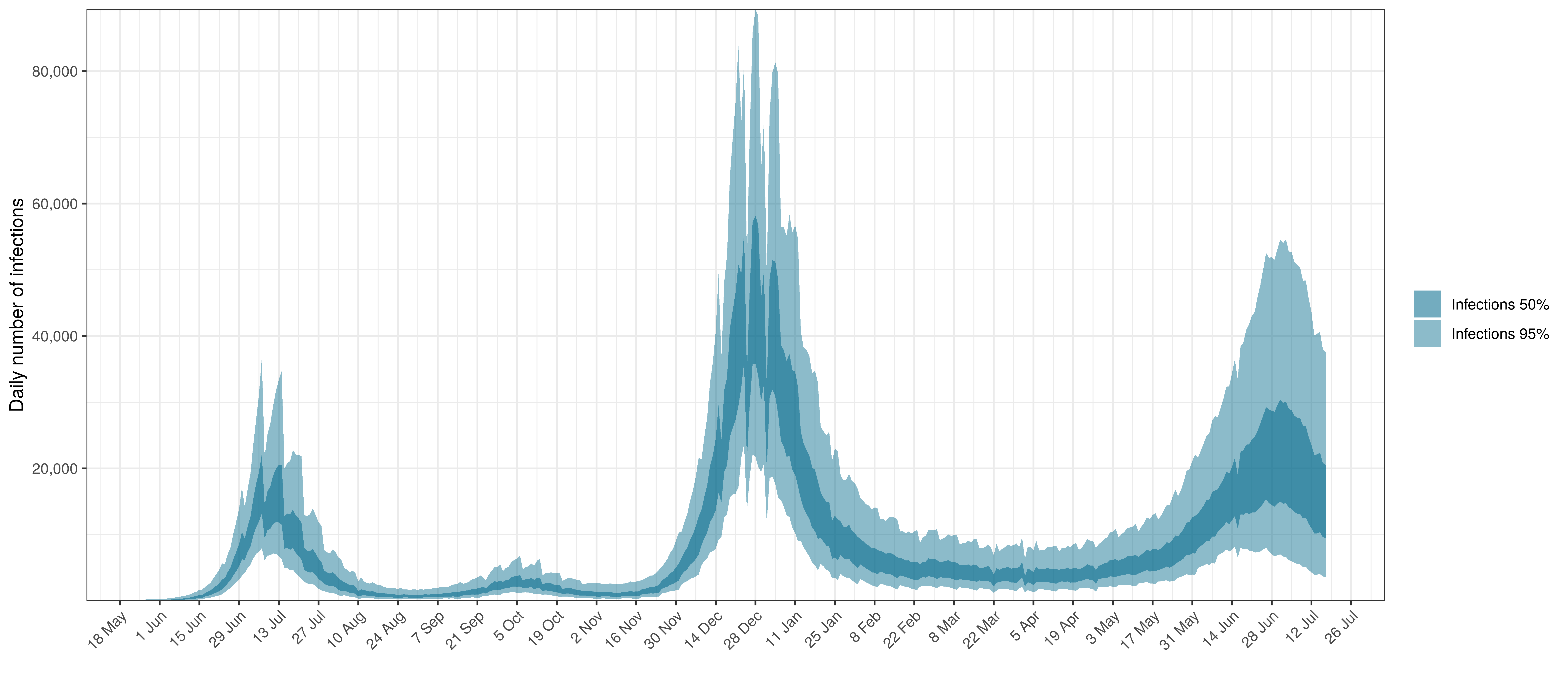
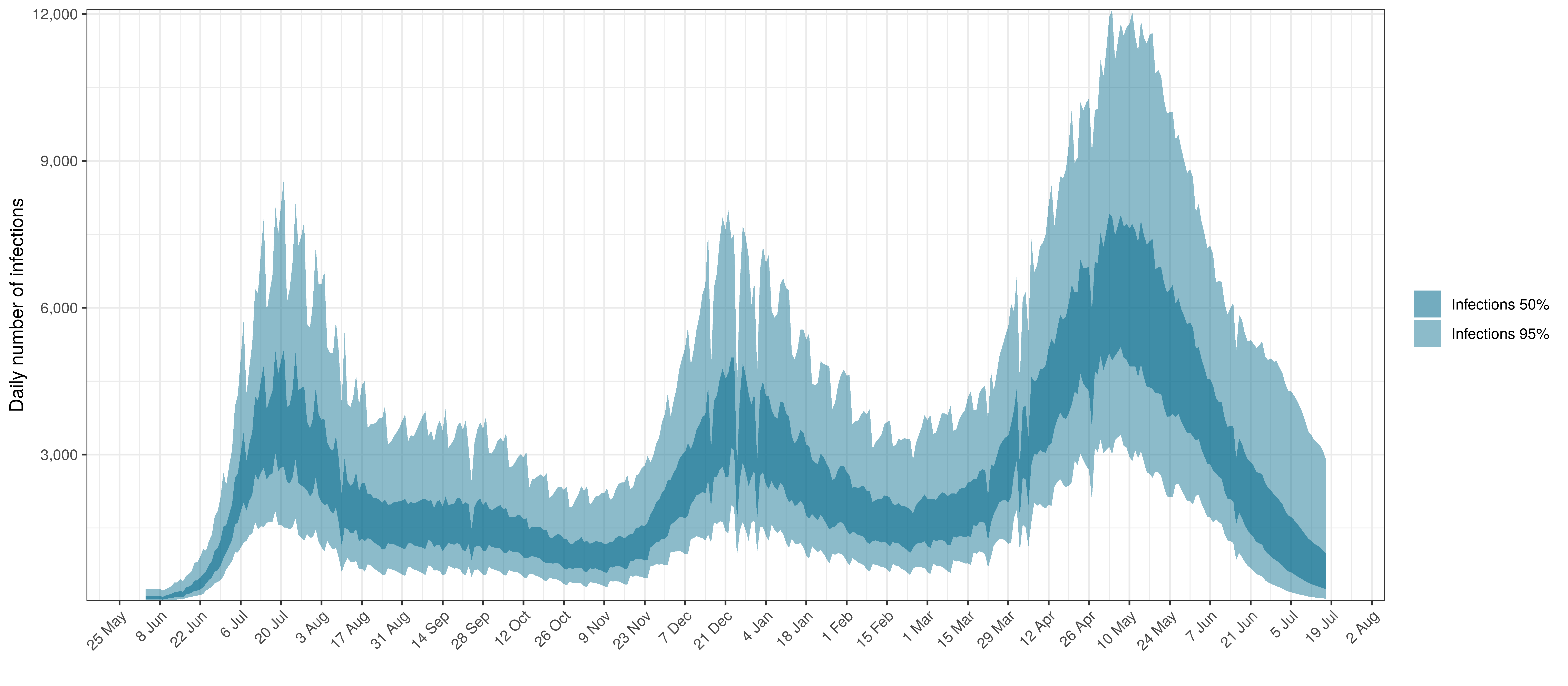
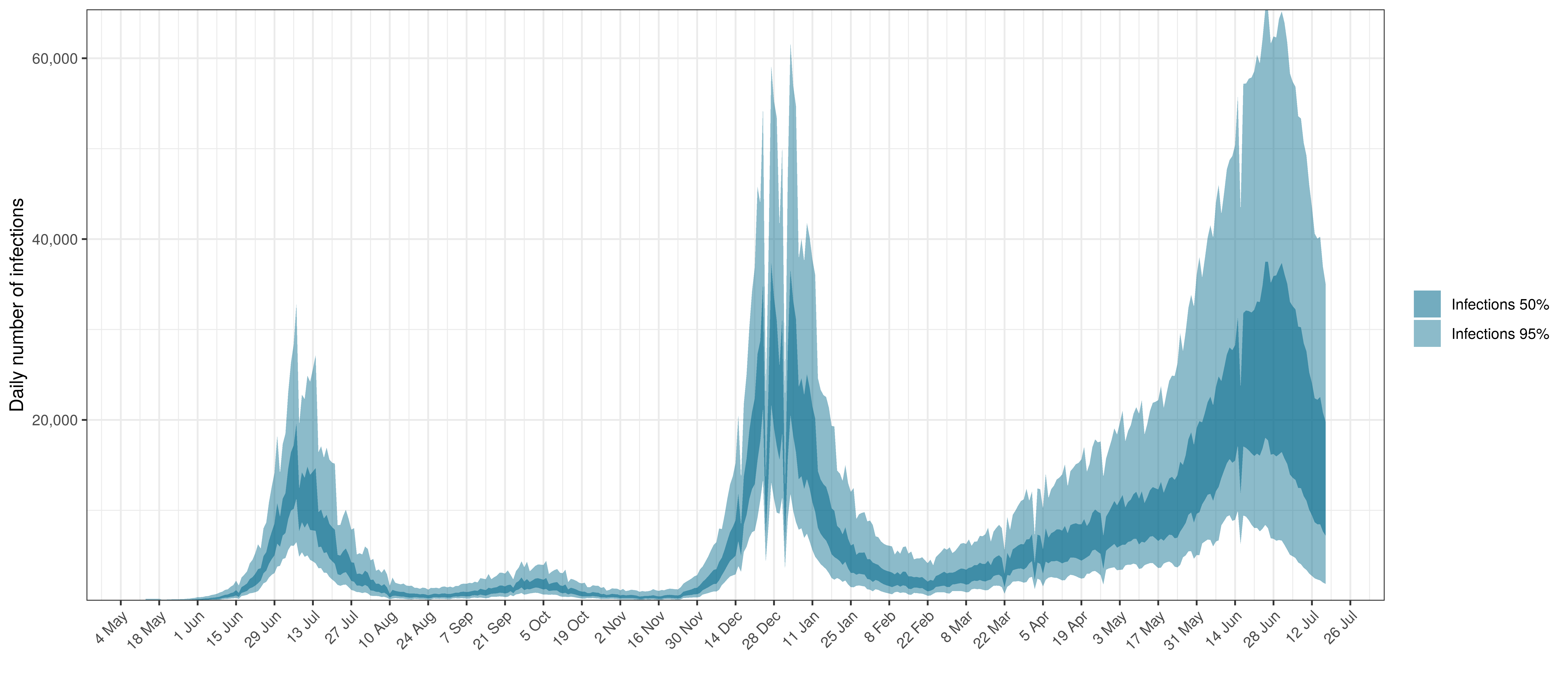
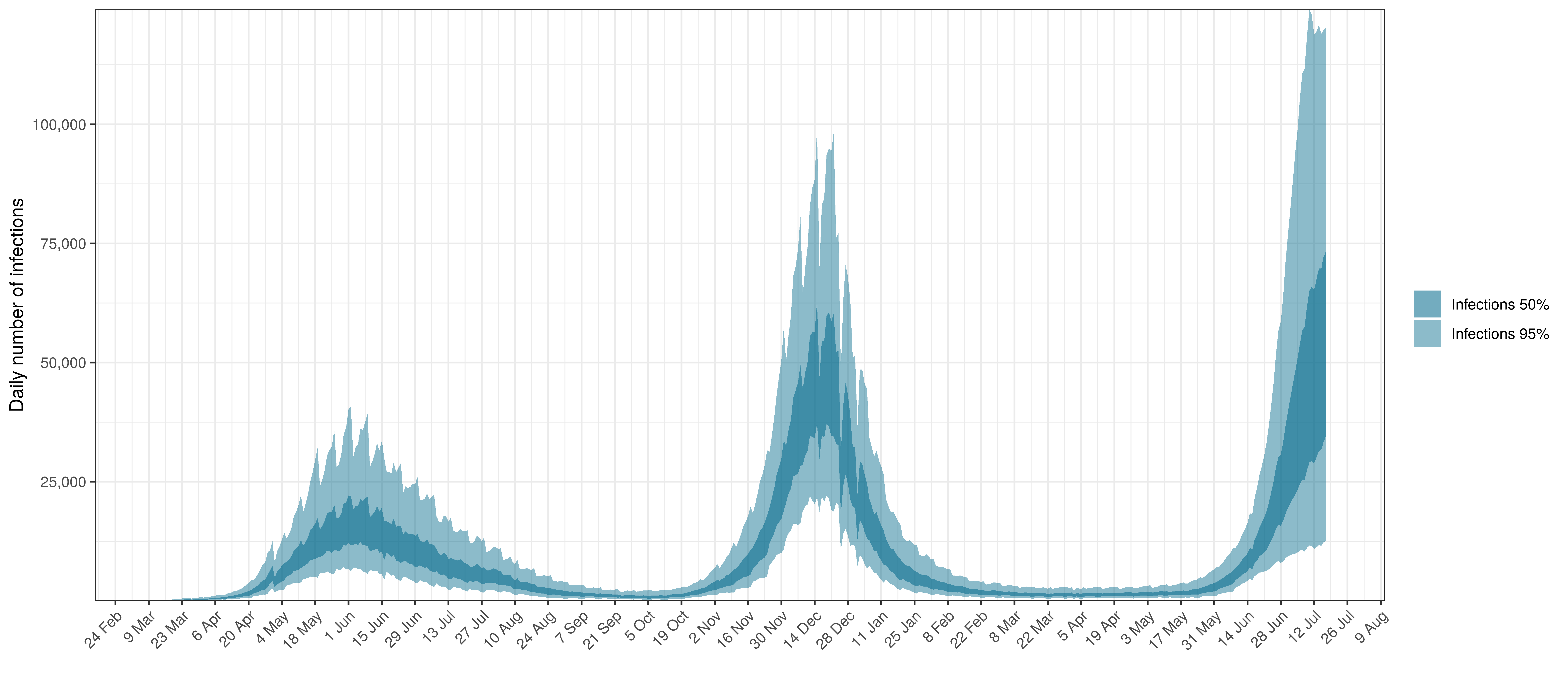
- The third panel shows the modelled daily number of infections (blue) compared to confirmed case counts (brown) as reported for the province. Note that this model does not calibrate to case data, but this data is shown for reference. We expect the model to produce infections exceeding confirmed cases as testing is likely only finding a fraction of the true infections.
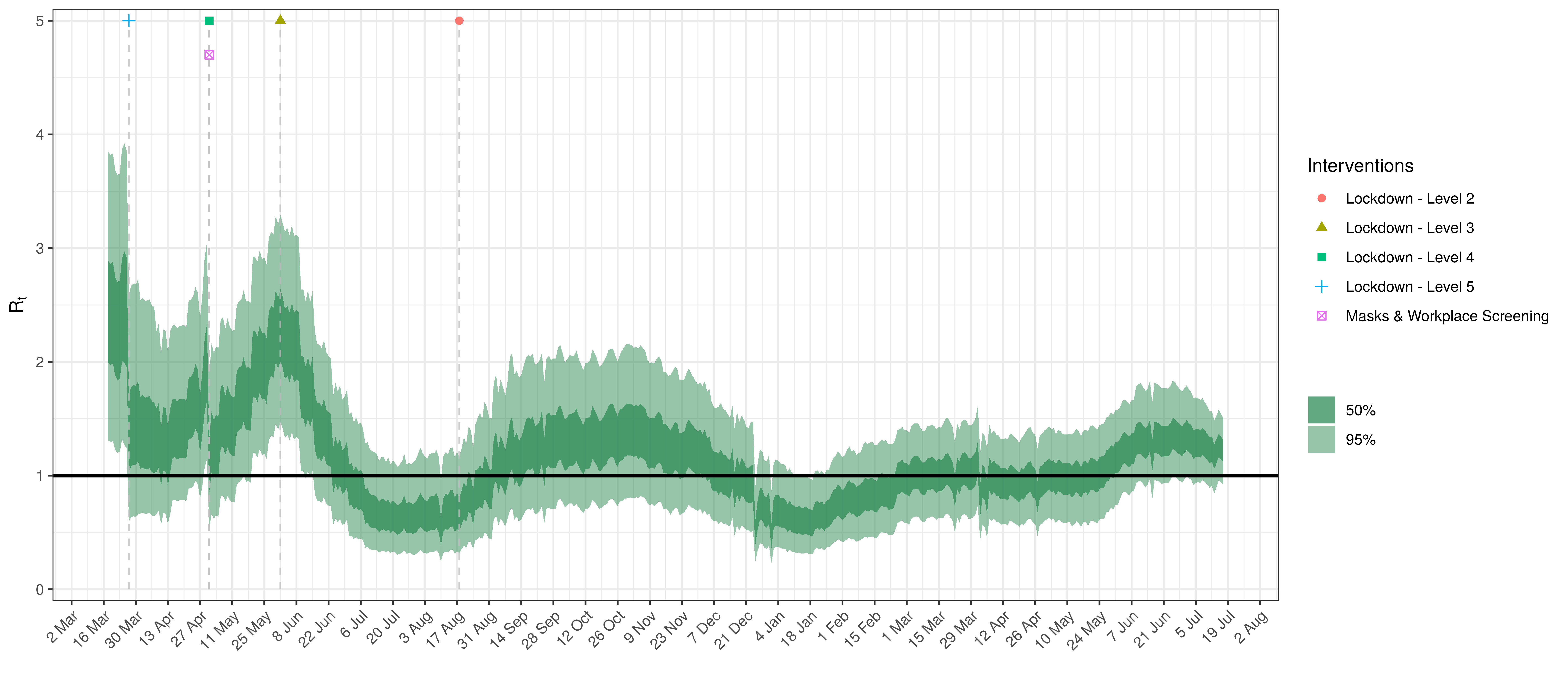
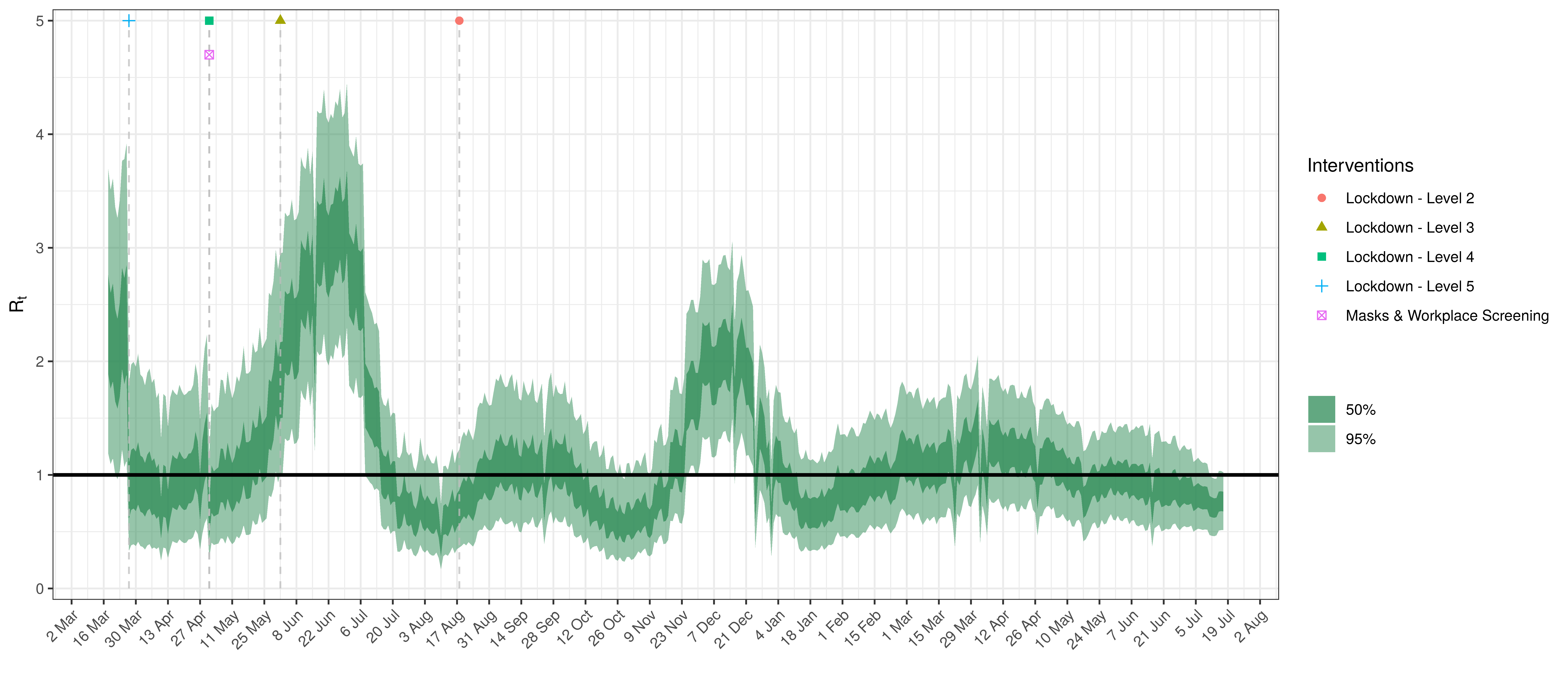
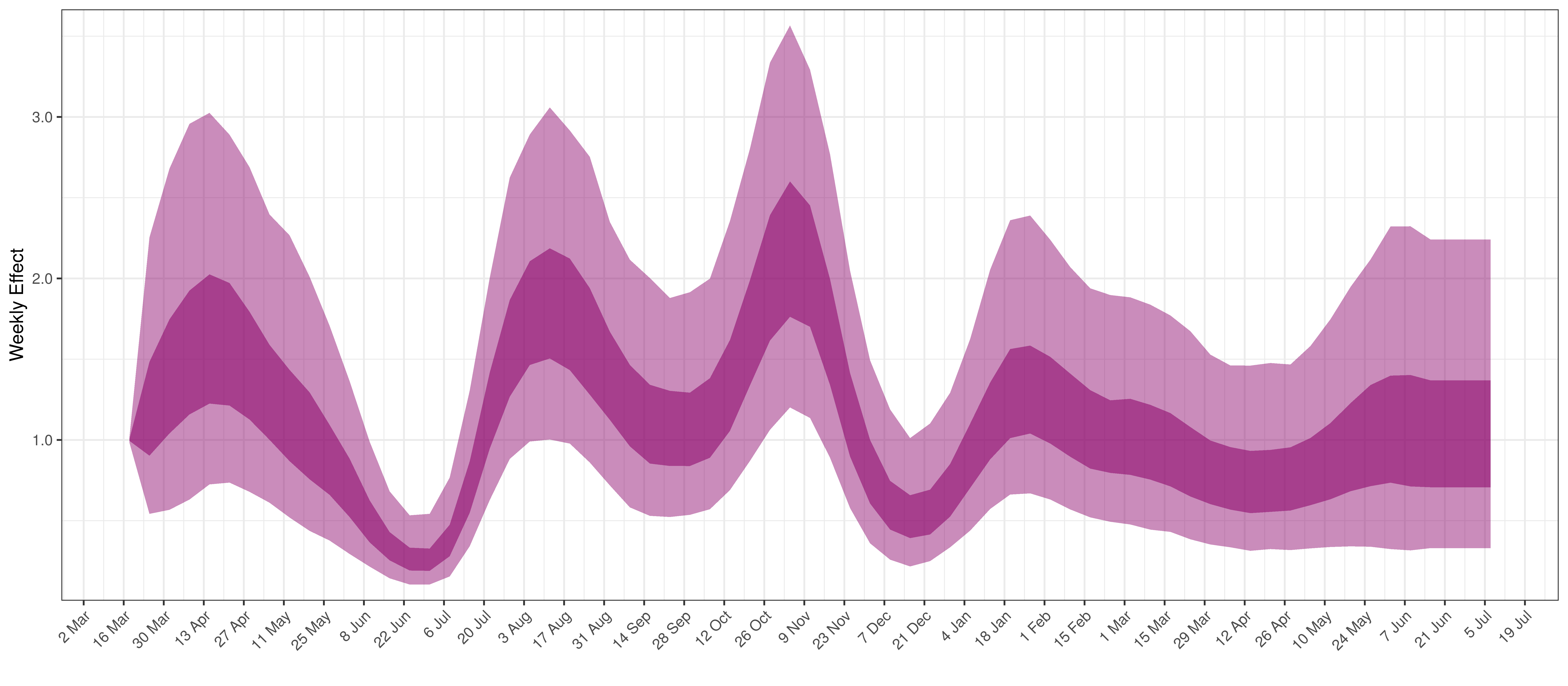
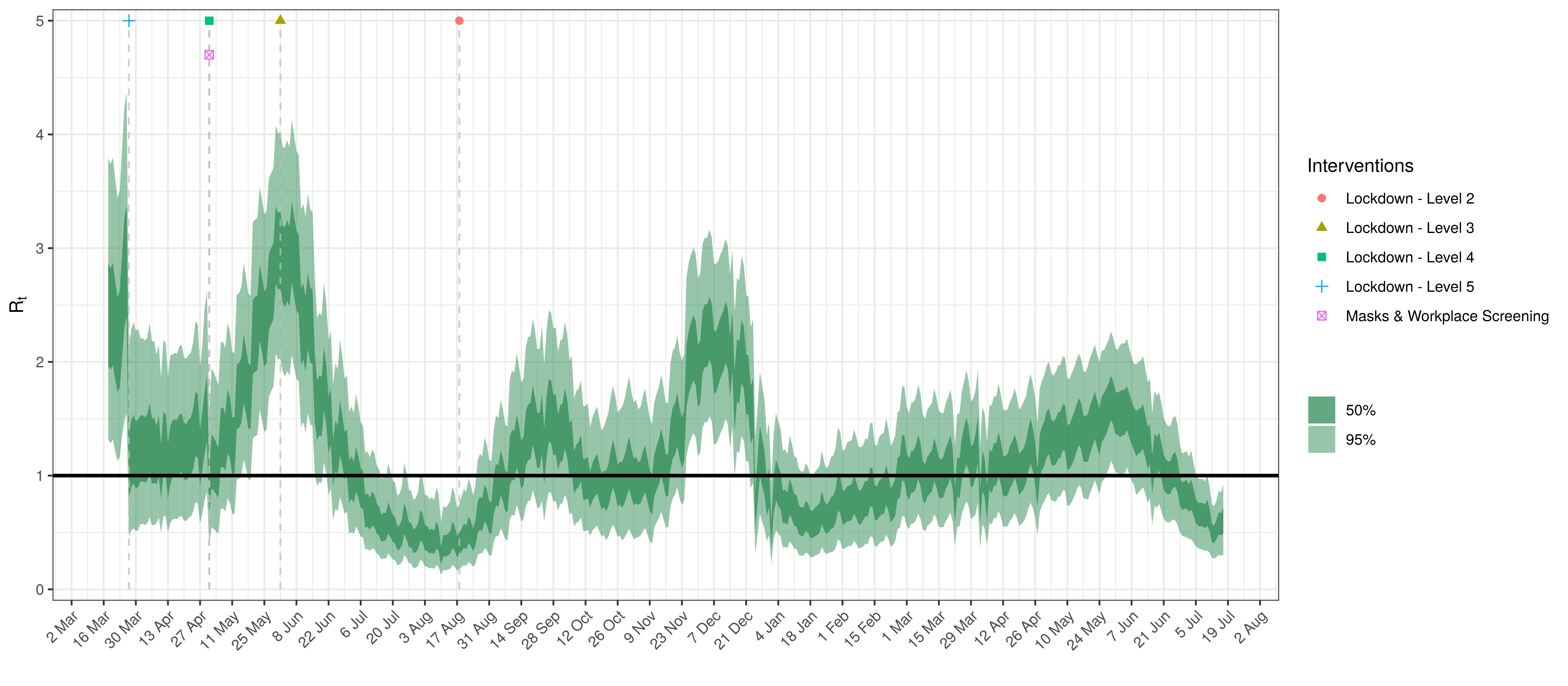
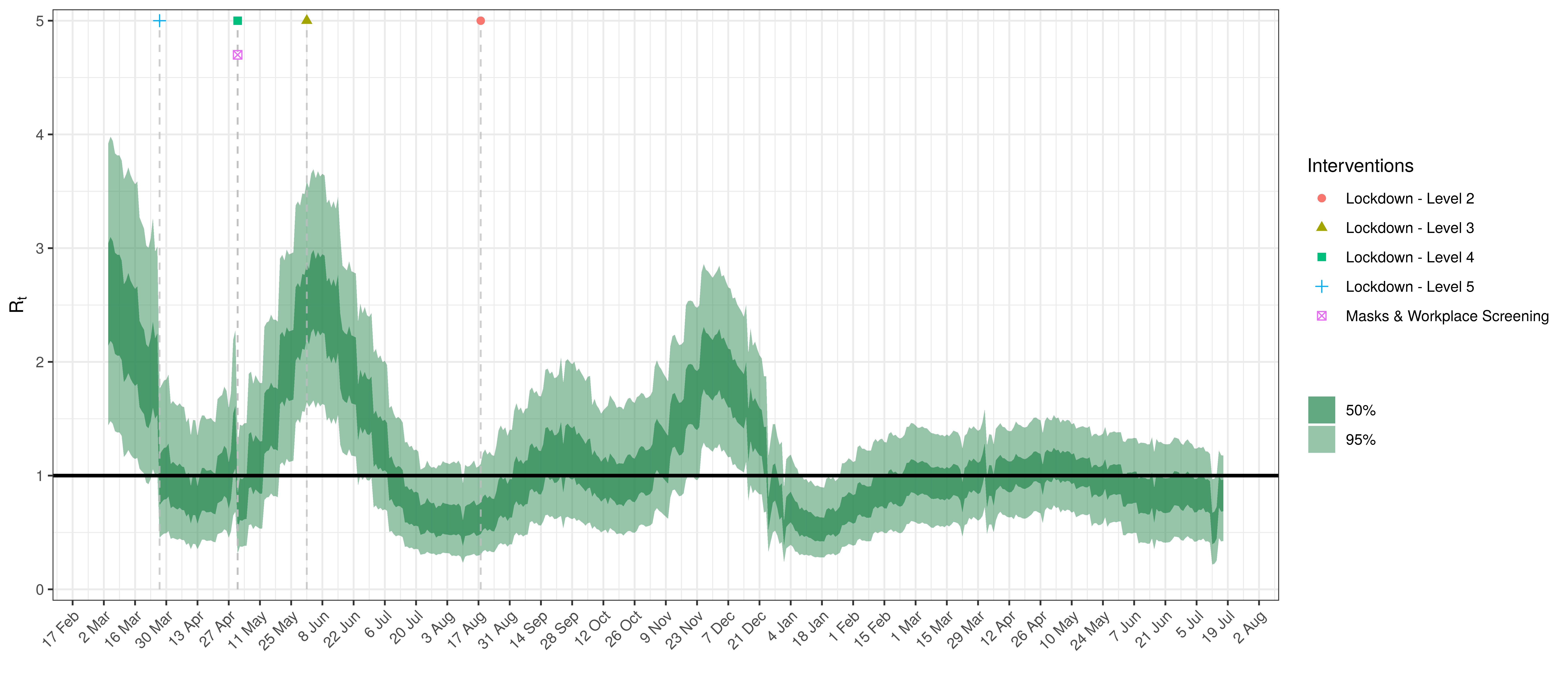
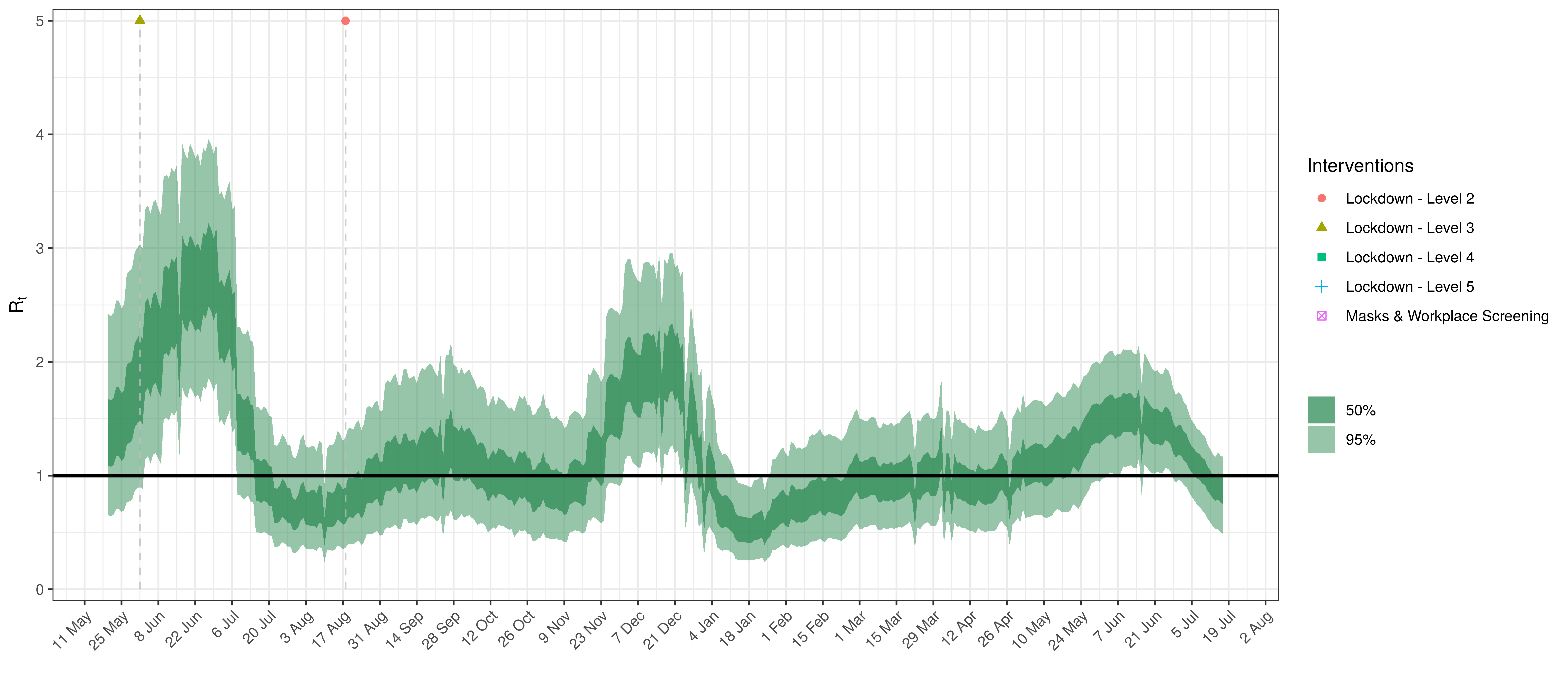
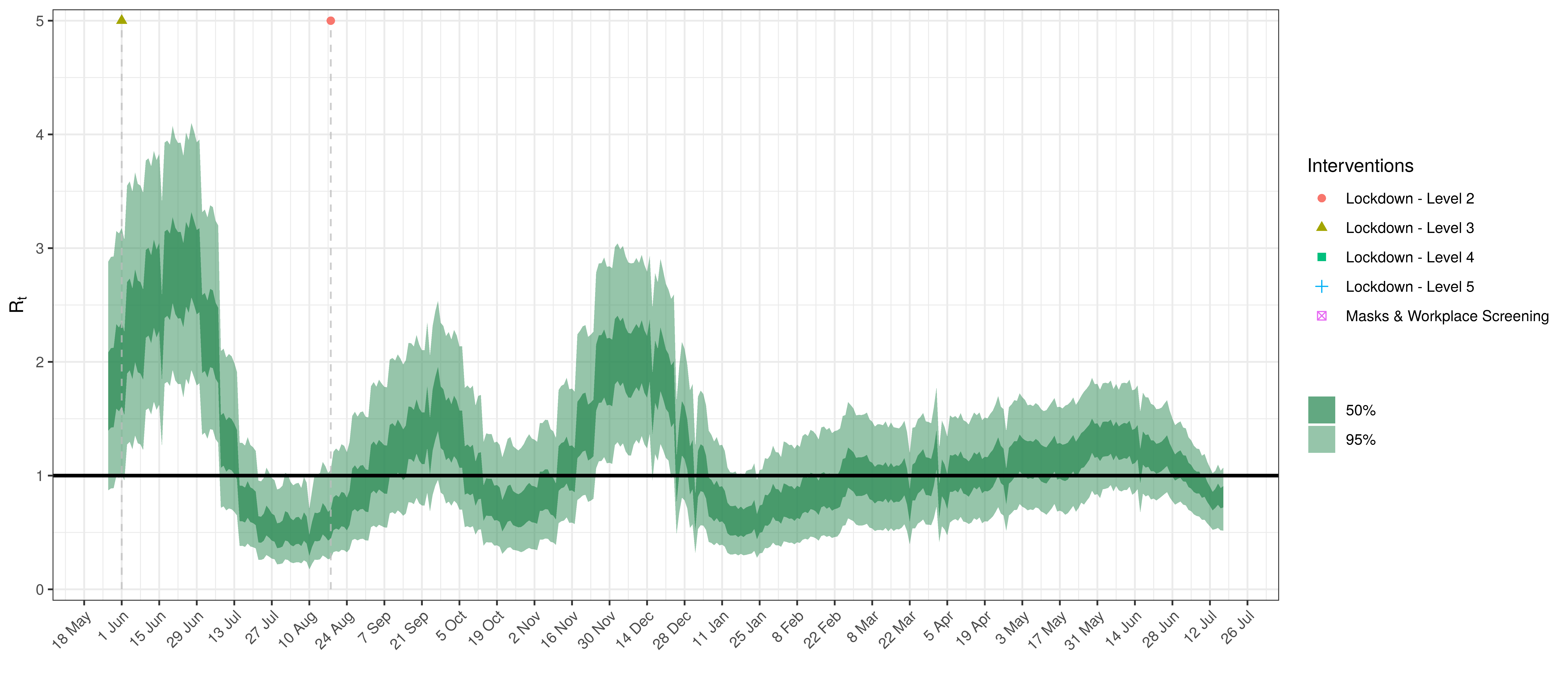
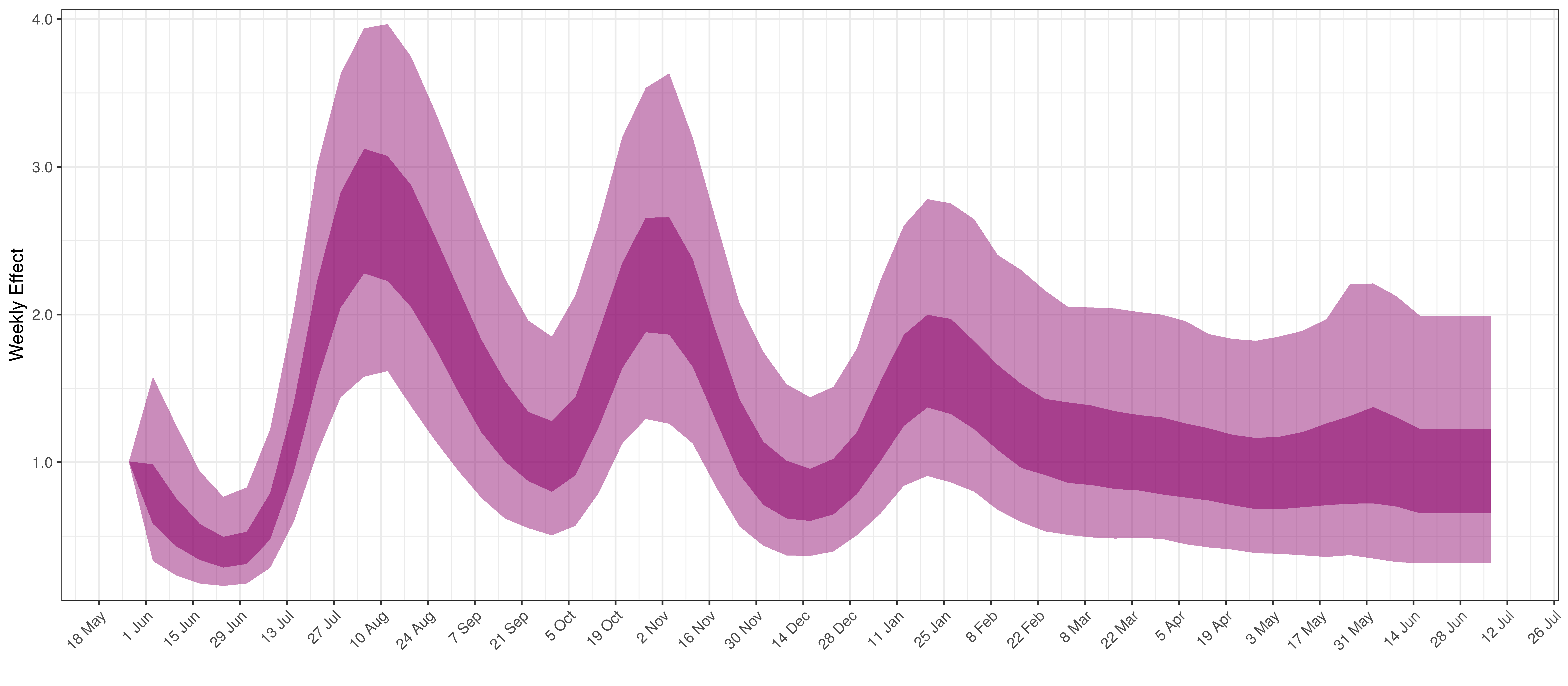
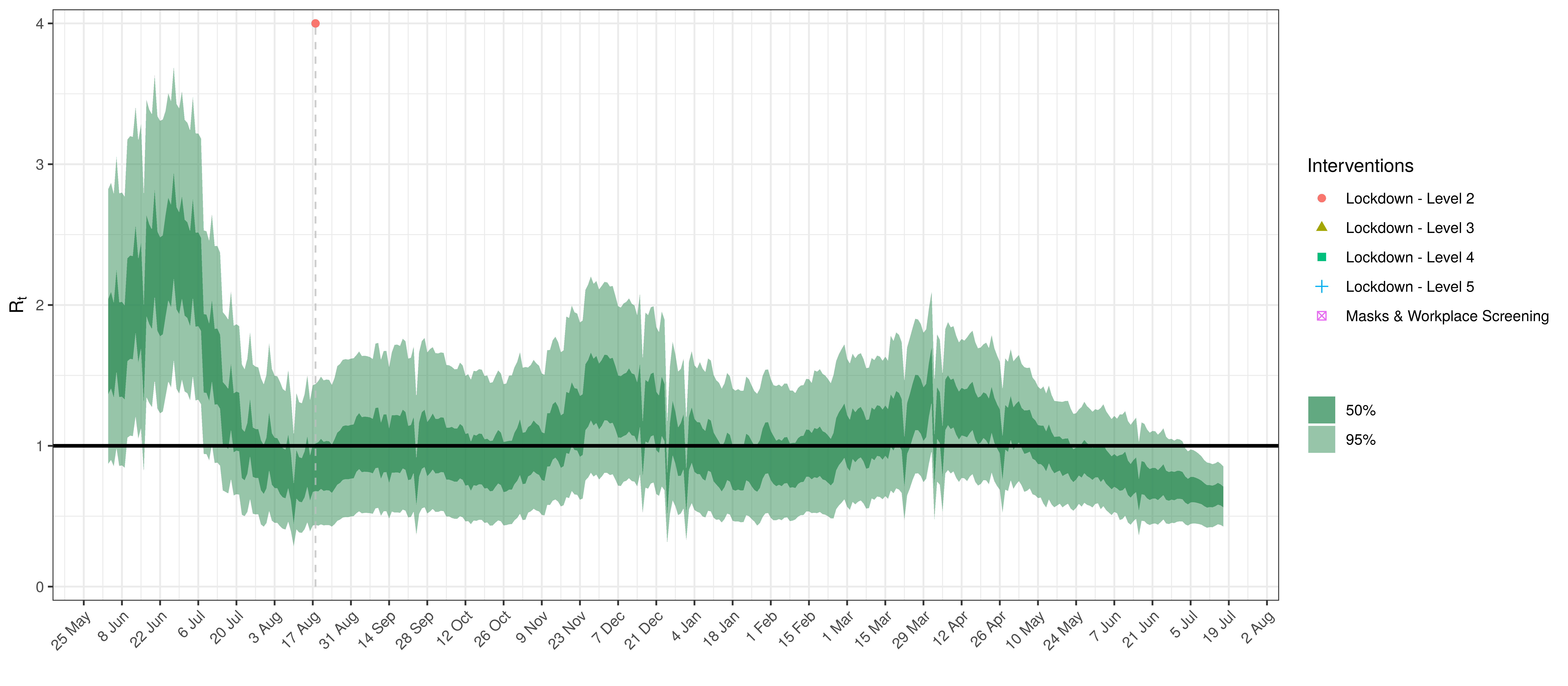
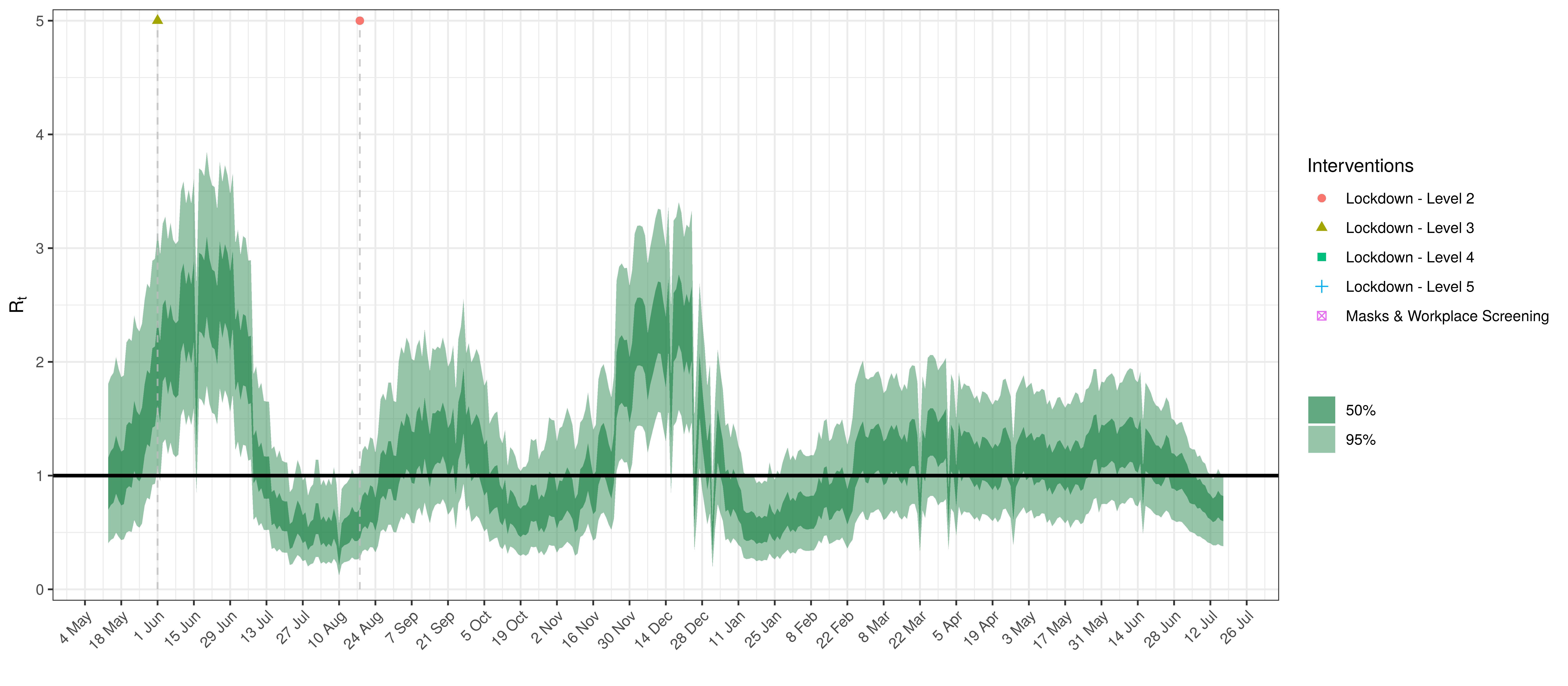
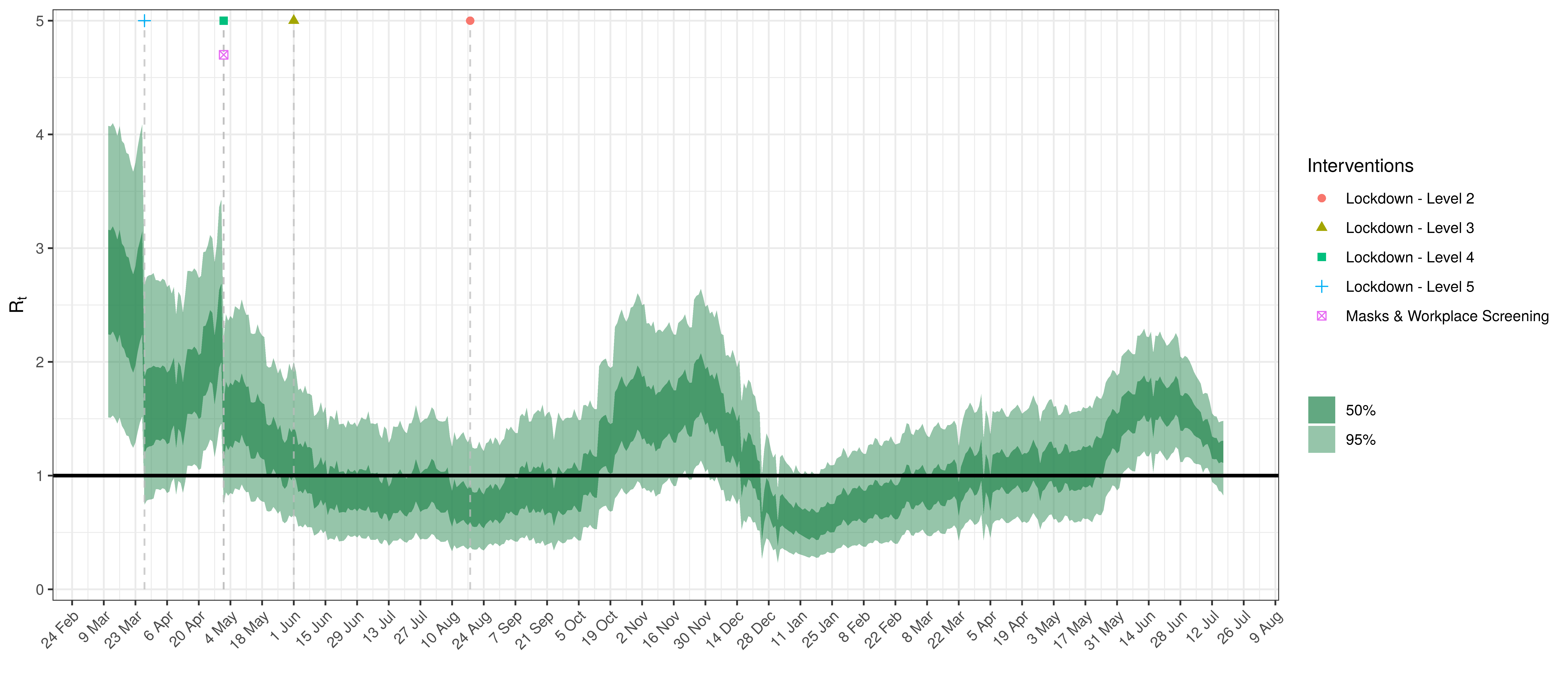
- The fourth panel shows the estimates for reproduction number (\(R_{t,m}\)) over time (\(t\)) for each province (\(m\)). These values are generating the infections in the model which result in deaths. Note that due to the delay of deaths following infections the last week or two of \(R_{t,m}\) values already present an extrapolation from the data. Deaths as a result of these recent infections have generally not occurred as yet.
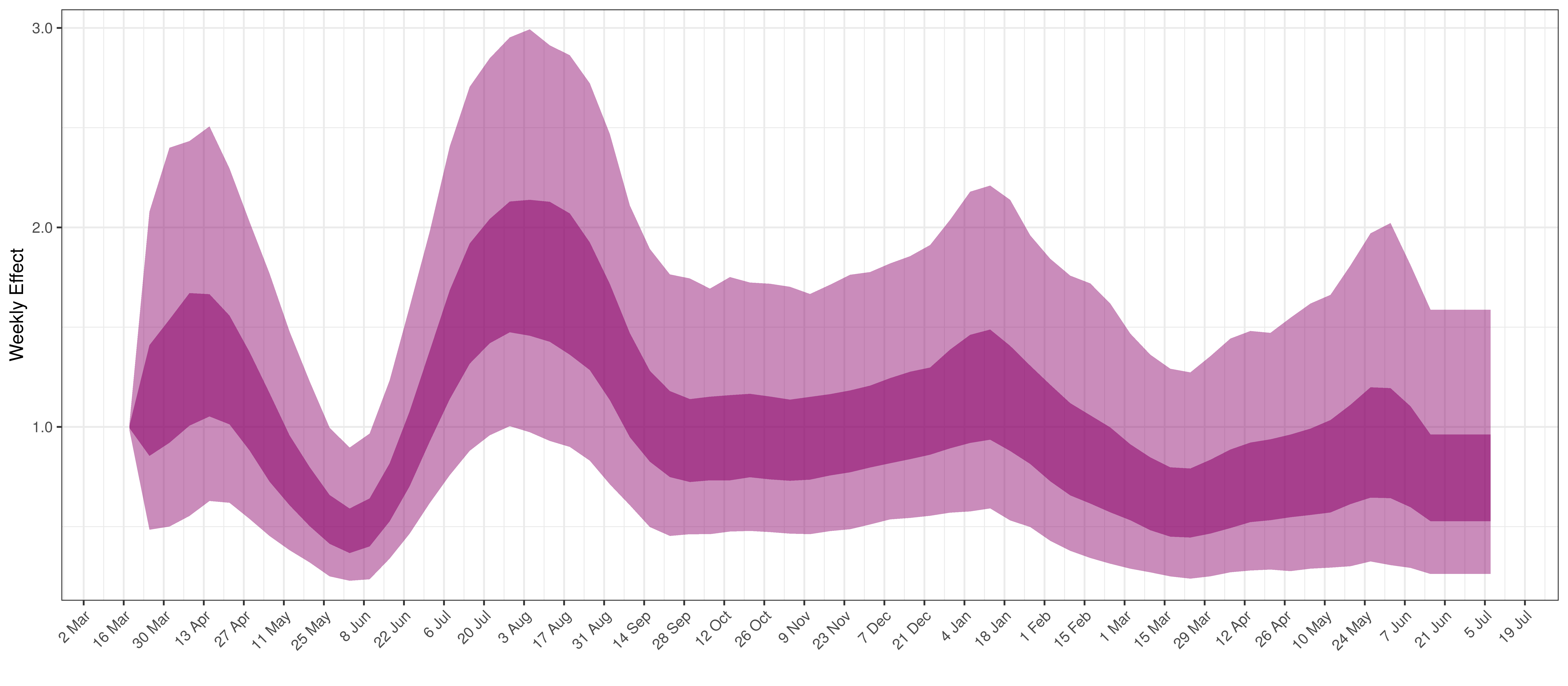
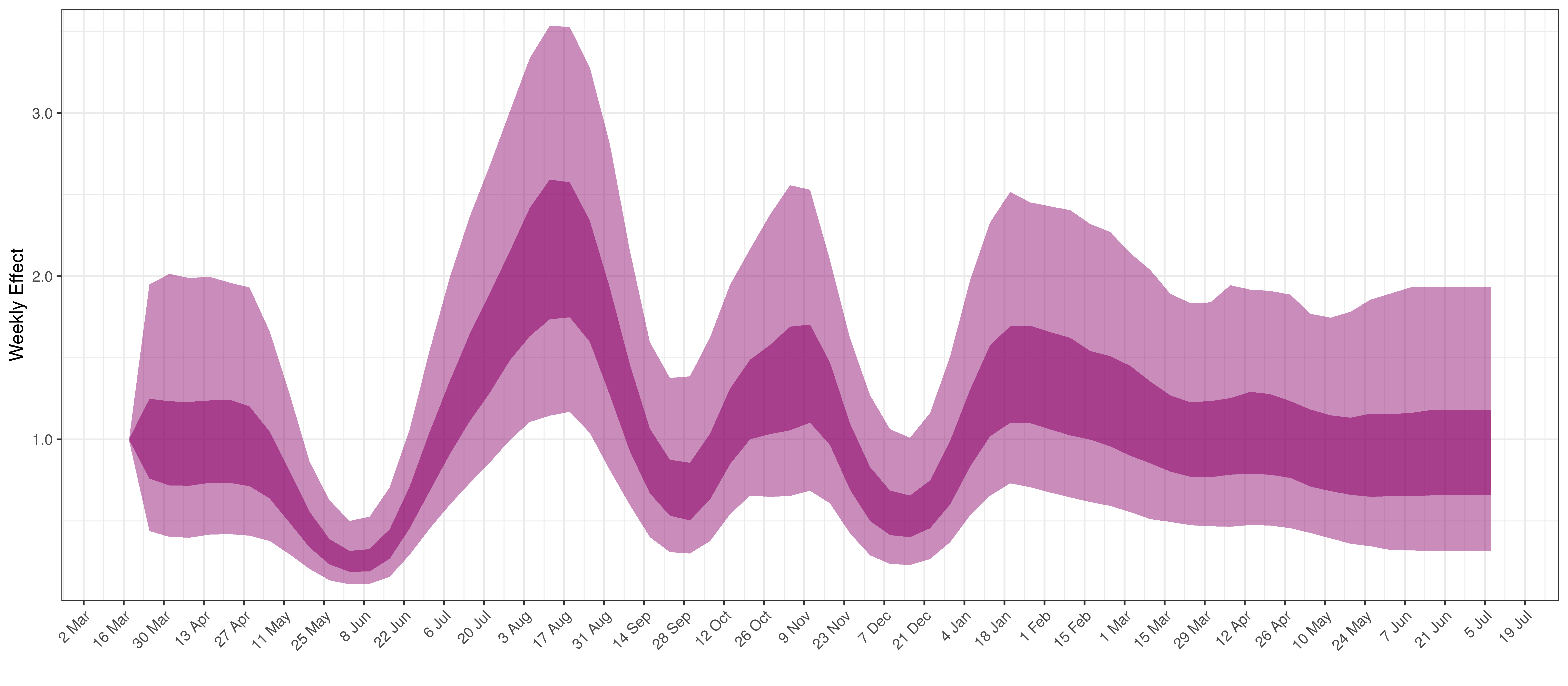
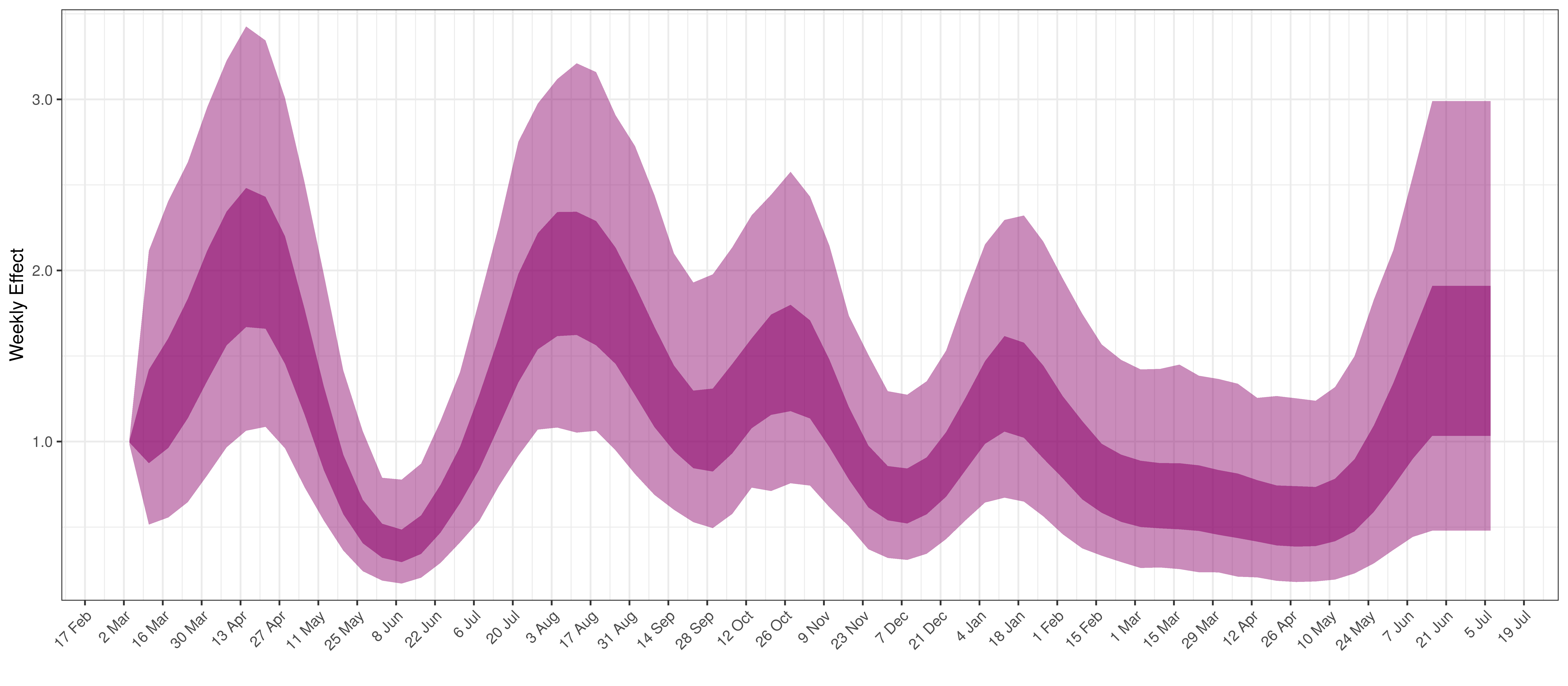
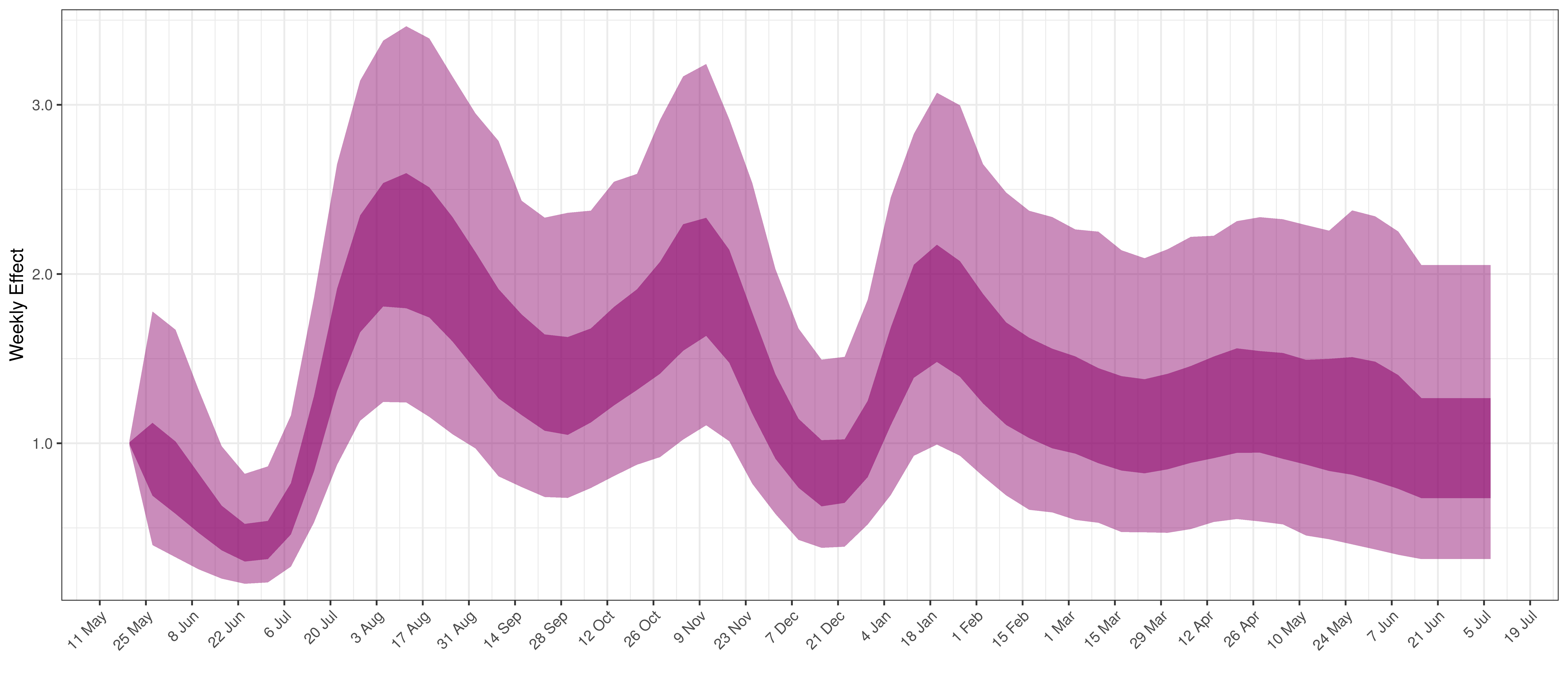
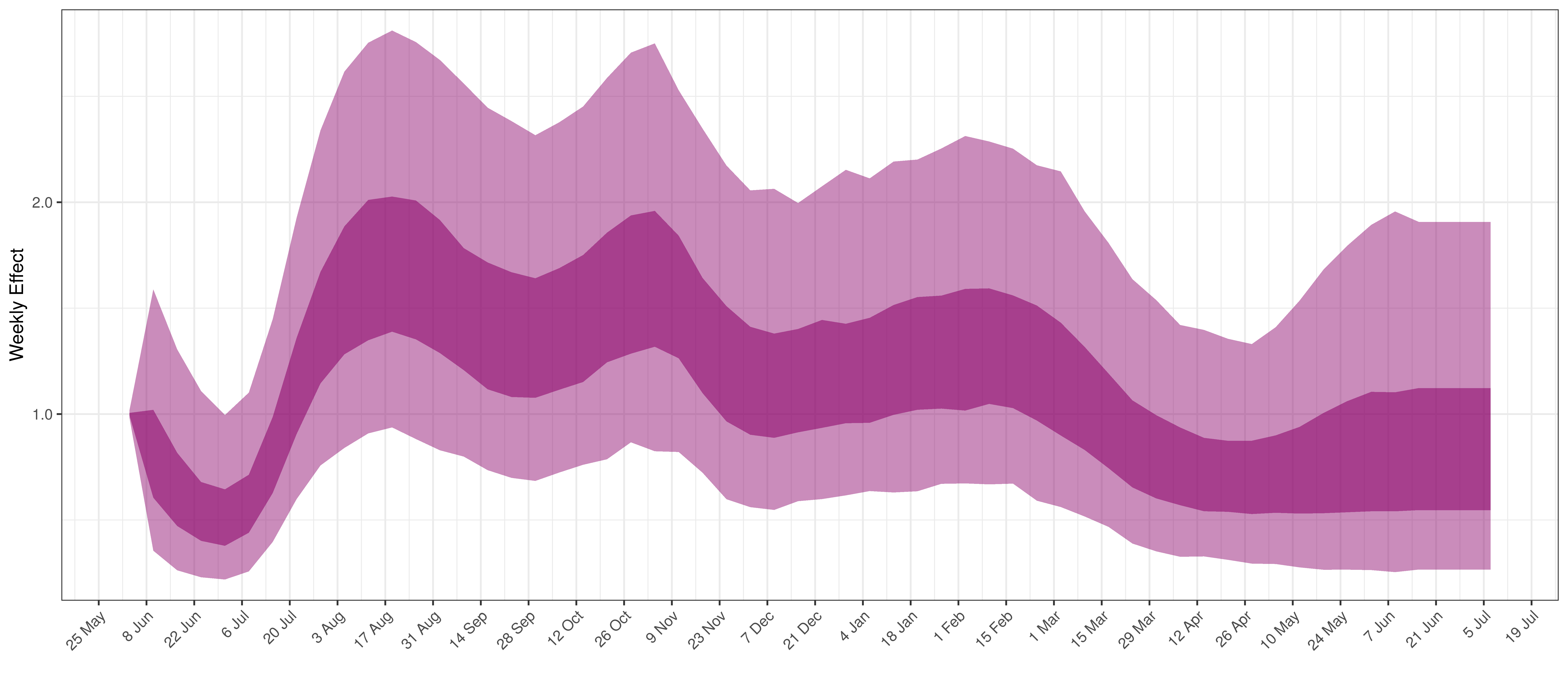
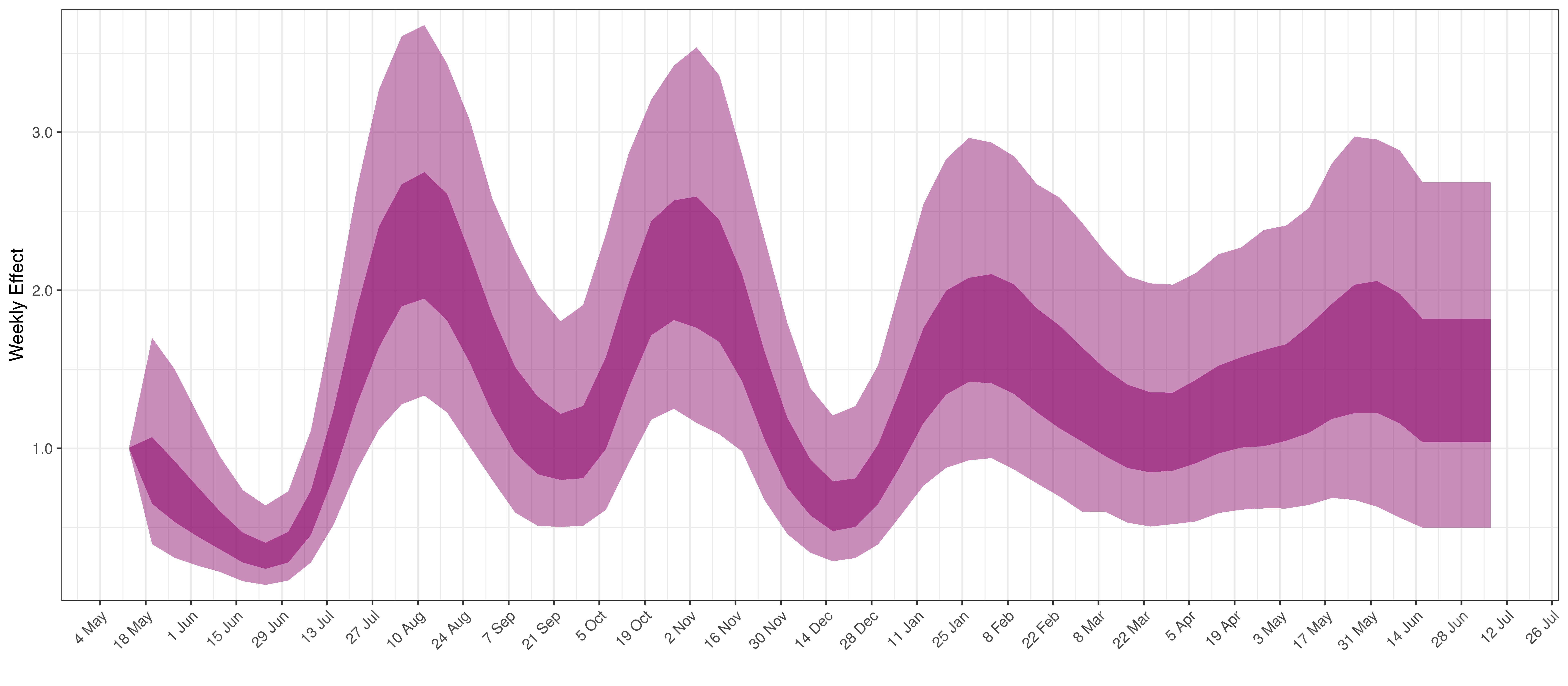
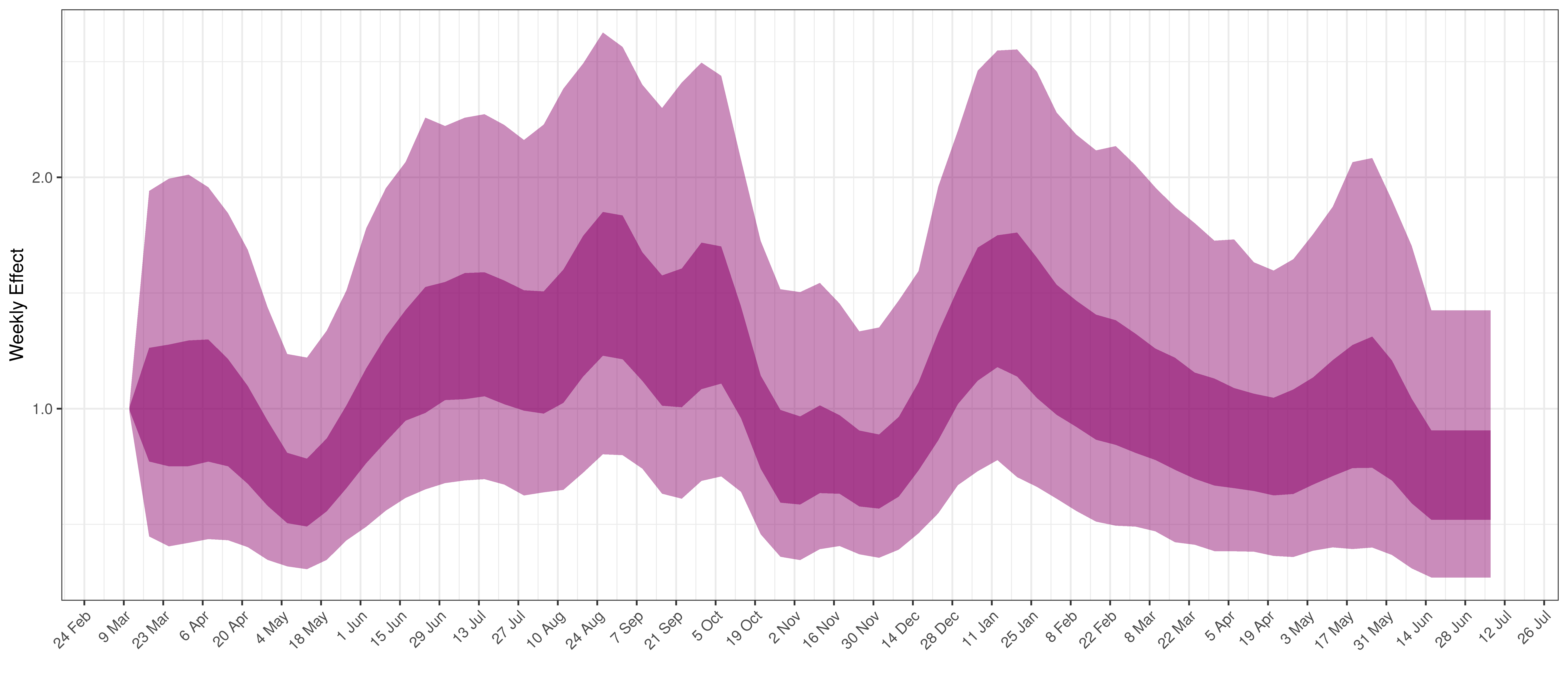
- The final panel shows the impact of the weekly AR(2) effect given a reproduction number of roughly 1. This unexplained value converted to a factor of \(R_{t,m}\). A value greater than 1 indicates that the \(R_{t,m}\) was higher than the value implied by other parameters. A value below 1 indicates the reverse.
In all the charts the darker shaded area represents a confidence interval of 50% and the lighter shaded area represents a confidence interval of 95%.
5.1 Eastern Cape
The chart below shows 90% of excess deaths and the modelled deaths.
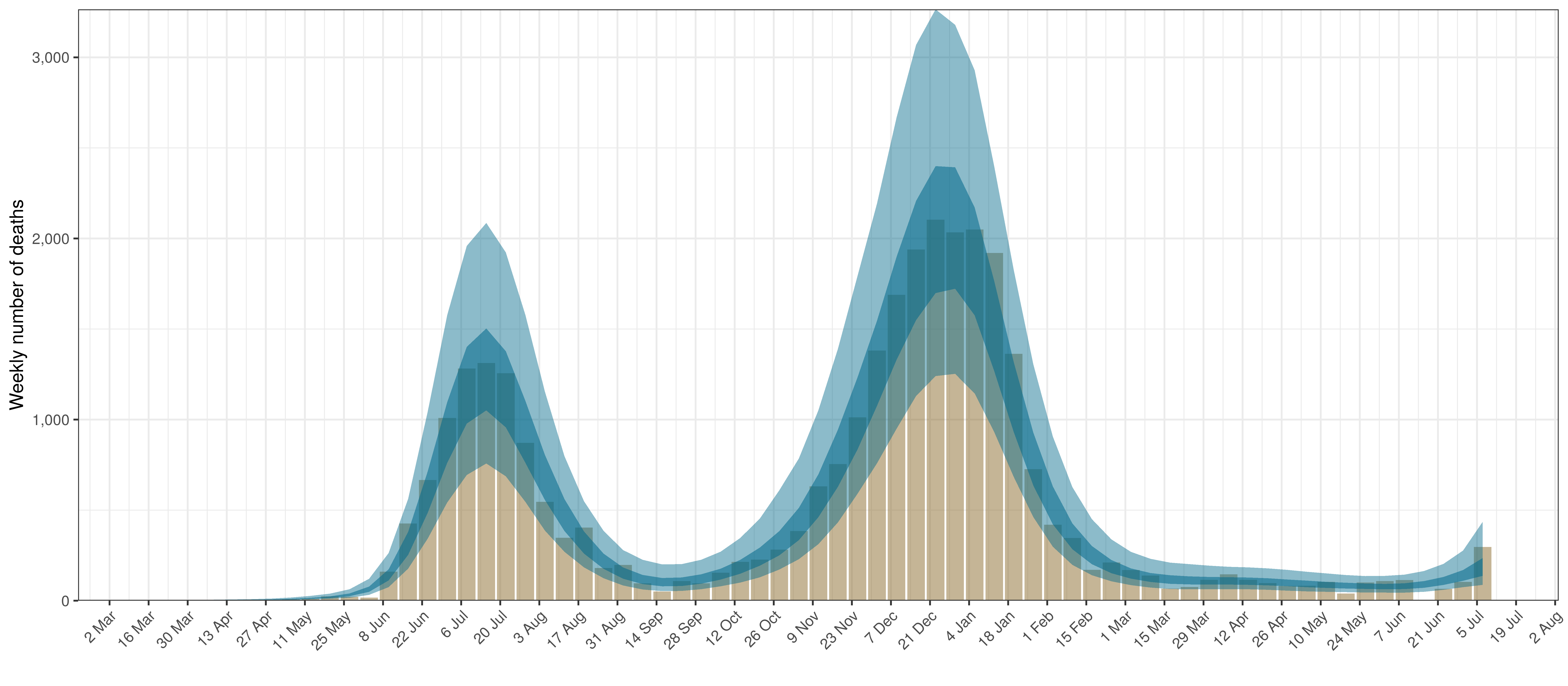
Projected Deaths and 90% of Excess Deaths in Eastern Cape
The reported deaths (in brown) and estimated deaths (in blue) are plotted below.
Projected Deaths compared to Reported COVID-19 Deaths in Eastern Cape
Below modelled infections are plotted compared to confirmed cases.
Projected Infections compared to Confirmed Cases in Eastern Cape
Below the \(R_{t,m}\) is plotted.
Effective Reproduction Number in Eastern Cape
Below the impact of the weekly AR(2) effect is plotted given a reproduction number of roughly 1.
Weekly AR(2) Factor Plot for Eastern Cape
5.2 Free State
The chart below shows 90% of excess deaths and the modelled deaths.
Projected Deaths and 90% of Excess Deaths in Free State
The reported deaths (in brown) and estimated deaths (in blue) are plotted below.
Projected Deaths compared to Reported COVID-19 Deaths in Free State
Below modelled infections are plotted compared to confirmed cases.
Projected Infections compared to Confirmed Cases in Free State
Below the \(R_{t,m}\) is plotted.
Effective Reproduction Number in Free State
Below the impact of the weekly AR(2) effect is plotted given a reproduction number of roughly 1.
Weekly AR(2) Factor Plot for Free State
5.3 Gauteng
The chart below shows 90% of excess deaths and the modelled deaths.
Projected Deaths and 90% of Excess Deaths in Gauteng
The reported deaths (in brown) and estimated deaths (in blue) are plotted below.
Projected Deaths compared to Reported COVID-19 Deaths in Gauteng
Below modelled infections are plotted compared to confirmed cases.
Projected Infections compared to Confirmed Cases in Gauteng
Below the \(R_{t,m}\) is plotted.
Effective Reproduction Number in Gauteng
Below the impact of the weekly AR(2) effect is plotted given a reproduction number of roughly 1.
Weekly AR(2) Factor Plot for Gauteng
5.4 KwaZulu-Natal
The chart below shows 90% of excess deaths and the modelled deaths.
Projected Deaths and 90% of Excess Deaths in KwaZulu-Natal
The reported deaths (in brown) and estimated deaths (in blue) are plotted below.
Projected Deaths compared to Reported COVID-19 Deaths in KwaZulu-Natal
Below modelled infections are plotted compared to confirmed cases.
Projected Infections compared to Confirmed Cases in KwaZulu-Natal
Below the \(R_{t,m}\) is plotted.
Effective Reproduction Number in KwaZulu-Natal
Below the impact of the weekly AR(2) effect is plotted given a reproduction number of roughly 1.
Weekly AR(2) Factor Plot for KwaZulu-Natal
5.5 Limpopo
The chart below shows 90% of excess deaths and the modelled deaths.
Projected Deaths and 90% of Excess Deaths in Limpopo
The reported deaths (in brown) and estimated deaths (in blue) are plotted below.
Projected Deaths compared to Reported COVID-19 Deaths in Limpopo
Below modelled infections are plotted compared to confirmed cases.
Projected Infections compared to Confirmed Cases in Limpopo
Below the \(R_{t,m}\) is plotted.
Effective Reproduction Number in Limpopo
Below the impact of the weekly AR(2) effect is plotted given a reproduction number of roughly 1.
Weekly AR(2) Factor Plot for Limpopo
5.6 Mpumalanga
The chart below shows 90% of excess deaths and the modelled deaths.
Projected Deaths and 90% of Excess Deaths in Mpumalanga
The reported deaths (in brown) and estimated deaths (in blue) are plotted below.
Projected Deaths compared to Reported COVID-19 Deaths in Mpumalanga
Below modelled infections are plotted compared to confirmed cases.
Projected Infections compared to Confirmed Cases in Mpumalanga
Below the \(R_{t,m}\) is plotted.
Effective Reproduction Number in Mpumalanga
Below the impact of the weekly AR(2) effect is plotted given a reproduction number of roughly 1.
Weekly AR(2) Factor Plot for Mpumalanga
5.7 Northern Cape
The chart below shows 90% of excess deaths and the modelled deaths.
Projected Deaths and 90% of Excess Deaths in Northern Cape
The reported deaths (in brown) and estimated deaths (in blue) are plotted below.
Projected Deaths compared to Reported COVID-19 Deaths in Northern Cape
Below modelled infections are plotted compared to confirmed cases.
Projected Infections compared to Confirmed Cases in Northern Cape
Below the \(R_{t,m}\) is plotted.
Effective Reproduction Number in Northern Cape
Below the impact of the weekly AR(2) effect is plotted given a reproduction number of roughly 1.
Weekly AR(2) Factor Plot for Northern Cape
5.8 North West
The chart below shows 90% of excess deaths and the modelled deaths.
Projected Deaths and 90% of Excess Deaths in North West
The reported deaths (in brown) and estimated deaths (in blue) are plotted below.
Projected Deaths compared to Reported COVID-19 Deaths in North West
Below modelled infections are plotted compared to confirmed cases.
Projected Infections compared to Confirmed Cases in North West
Below the \(R_{t,m}\) is plotted.
Effective Reproduction Number in North West
Below the impact of the weekly AR(2) effect is plotted given a reproduction number of roughly 1.
Weekly AR(2) Factor Plot for North West
5.9 Western Cape
The chart below shows 90% of excess deaths and the modelled deaths.
Projected Deaths and 90% of Excess Deaths in Western Cape
The reported deaths (in brown) and estimated deaths (in blue) are plotted below.
Projected Deaths compared to Reported COVID-19 Deaths in Western Cape
Below modelled infections are plotted compared to confirmed cases.
Projected Infections compared to Confirmed Cases in Western Cape
Below the \(R_{t,m}\) is plotted.
Effective Reproduction Number in Western Cape
Below the impact of the weekly AR(2) effect is plotted given a reproduction number of roughly 1.
Weekly AR(2) Factor Plot for Western Cape
6 Parameter Estimates
Below we plot the percentage reduction in \(R_{t,m}\) assuming all other effects in the model are 0 except for the impact of interventions introduced with Level 4 (including mask-wearing and workplace screening). This is equivalent to plotting \(1-2\cdot\phi^{-1}(-\beta)\).
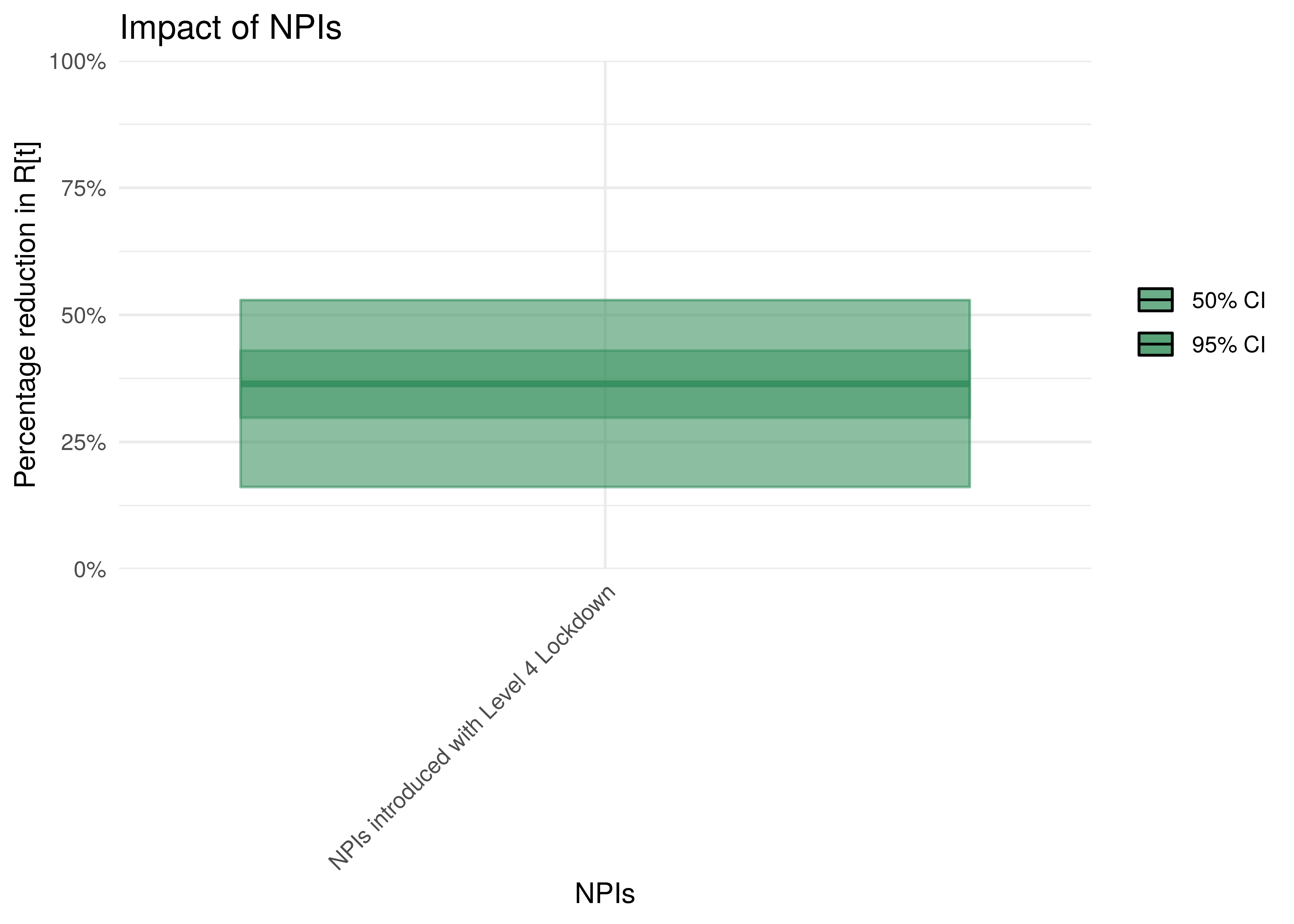
Impact of interventions introduced with Level 4
To understand the impact of mobility, the percentage reduction in \(R_{t,m}\) due to a mobility index of 0.1 is plotted. The assumption is that \(R_{t,m}=1\) before the reduction.
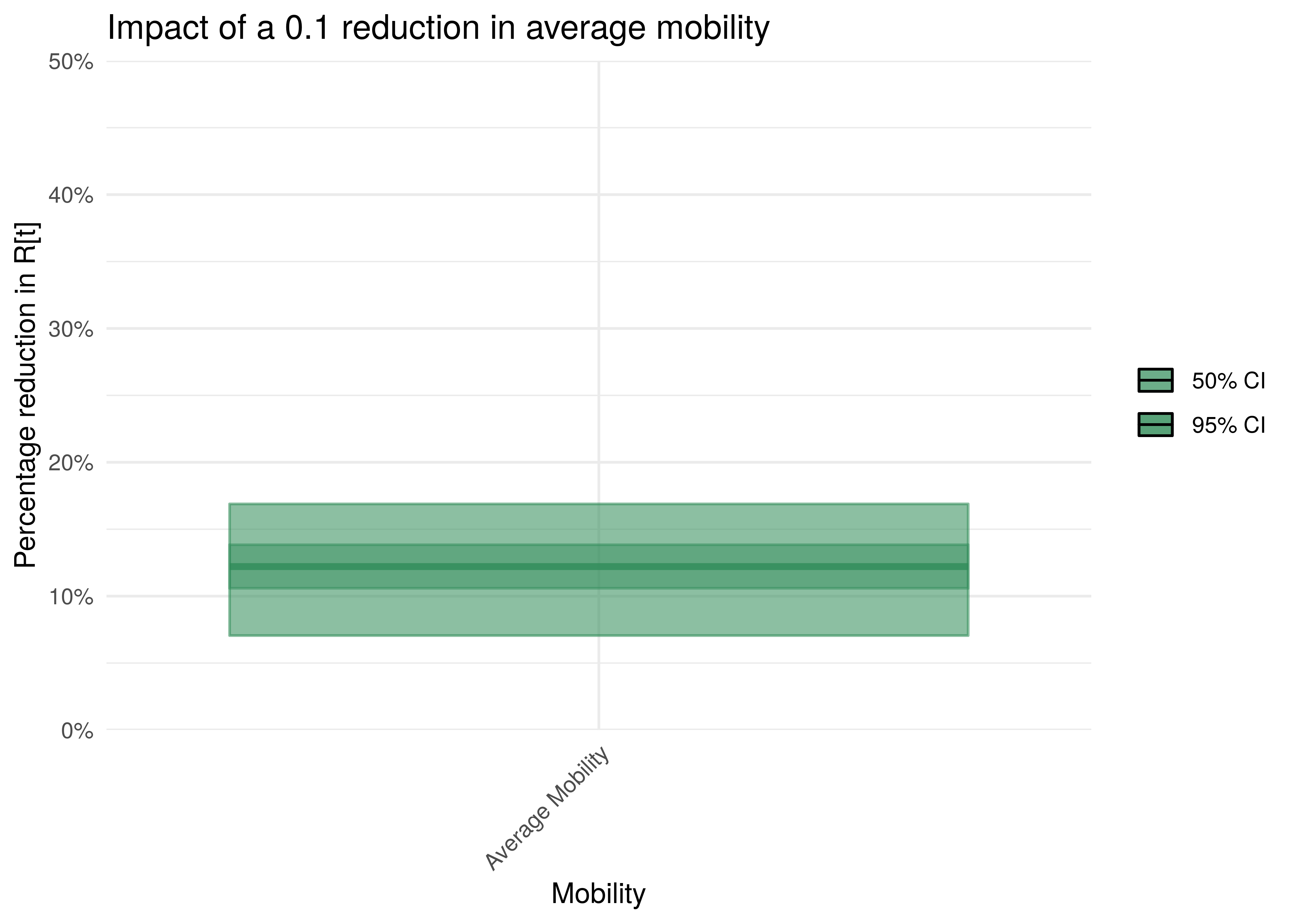
Impact of 0.1 reduction in mobility
To understand the net parameter estimates for \(\delta\) (the impact of the variants) we plot the percentage increase in \(R_{t,m}\) from 1 assuming the particular variant is dominant.
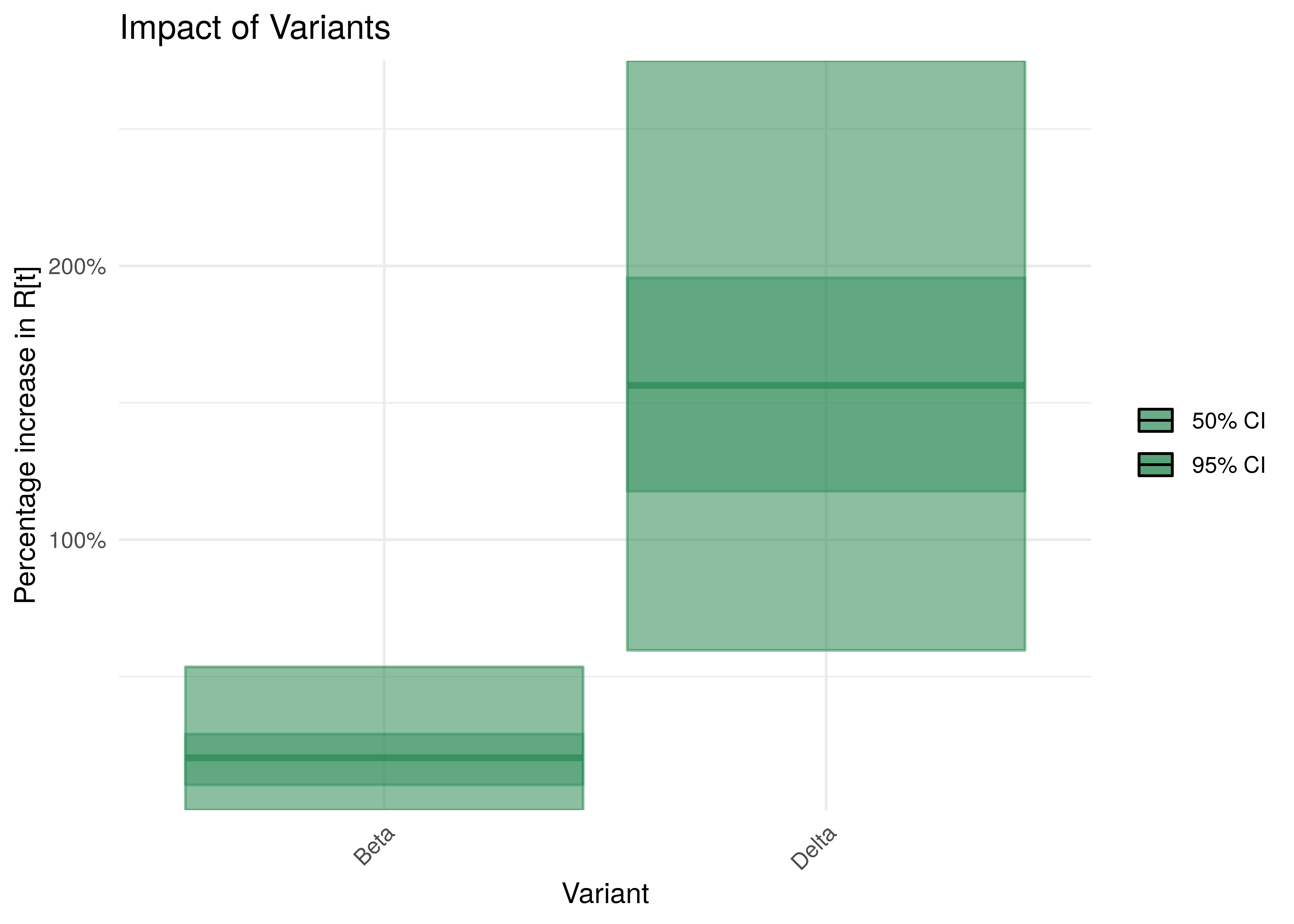
Impact of Variants with 95% Confidence Intervals
7 Reproduction Number Estimates
7.1 Initial Reproduction Number
Estimates for \(R_{0,m}\) for each province are plotted below. In all provinces posterior estimates for \(R_{0,m}\) are not heavily influenced by the data. This is probably due to the relatively early lockdown implemented in South Africa. This has thus been set to a single value that’s the same across all provinces and hence the plots
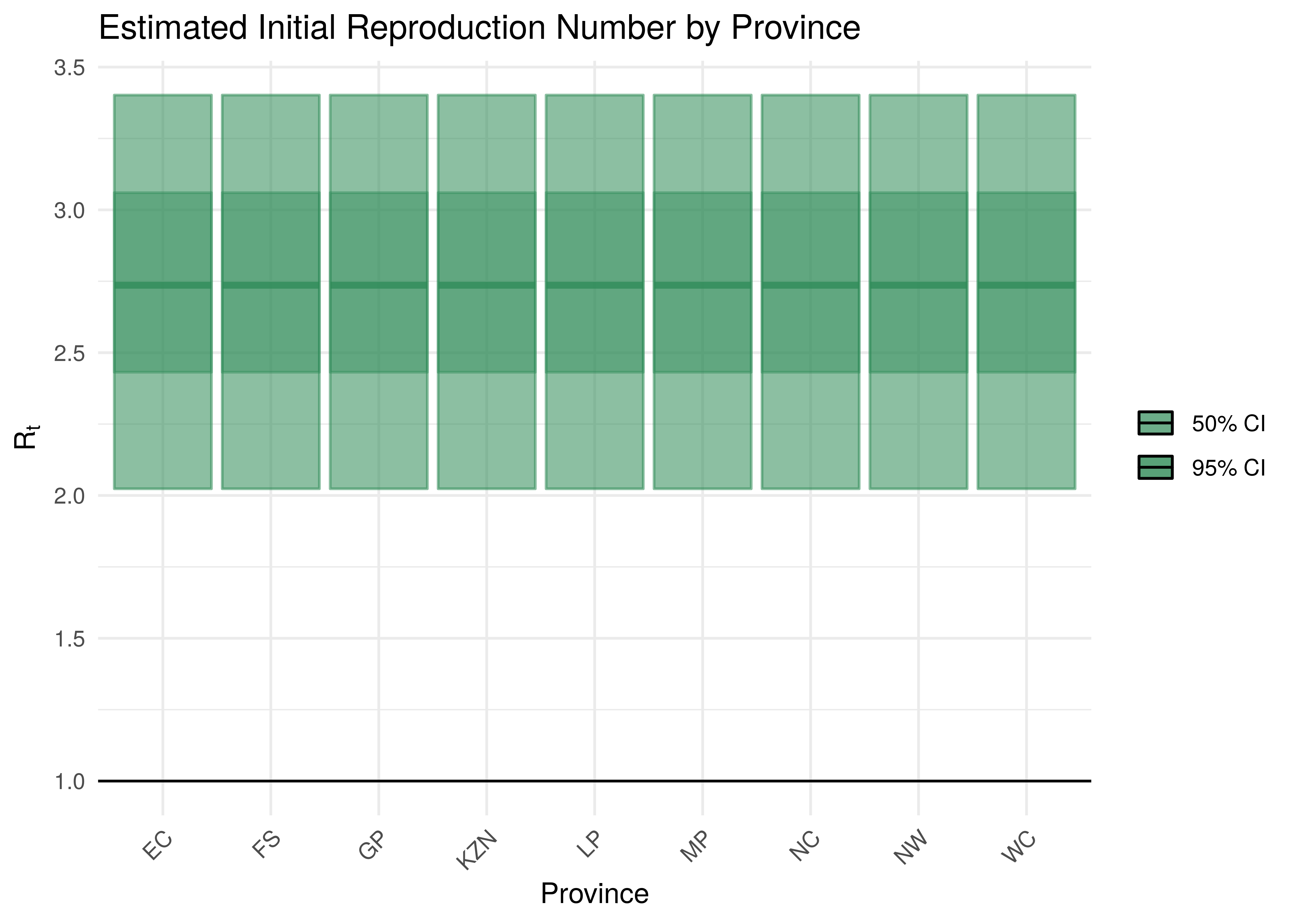
Initial Reproduction Number by Province
7.2 Current Reproduction Number as at 17 July 2021
Current estimates and 95% confidence intervals for \(R_{t,m}\) (current effective reproduction number) are plotted below for each province. A value below 1 would indicate an epidemic that is slowing while a value above 1 indicates an epidemic that is growing. It is clear that the spread of the epidemic is somewhat slowed compared to the initial \(R_{0,m}\). For some provinces the confidence interval does not include 1 which would indicate this to a stronger degree.
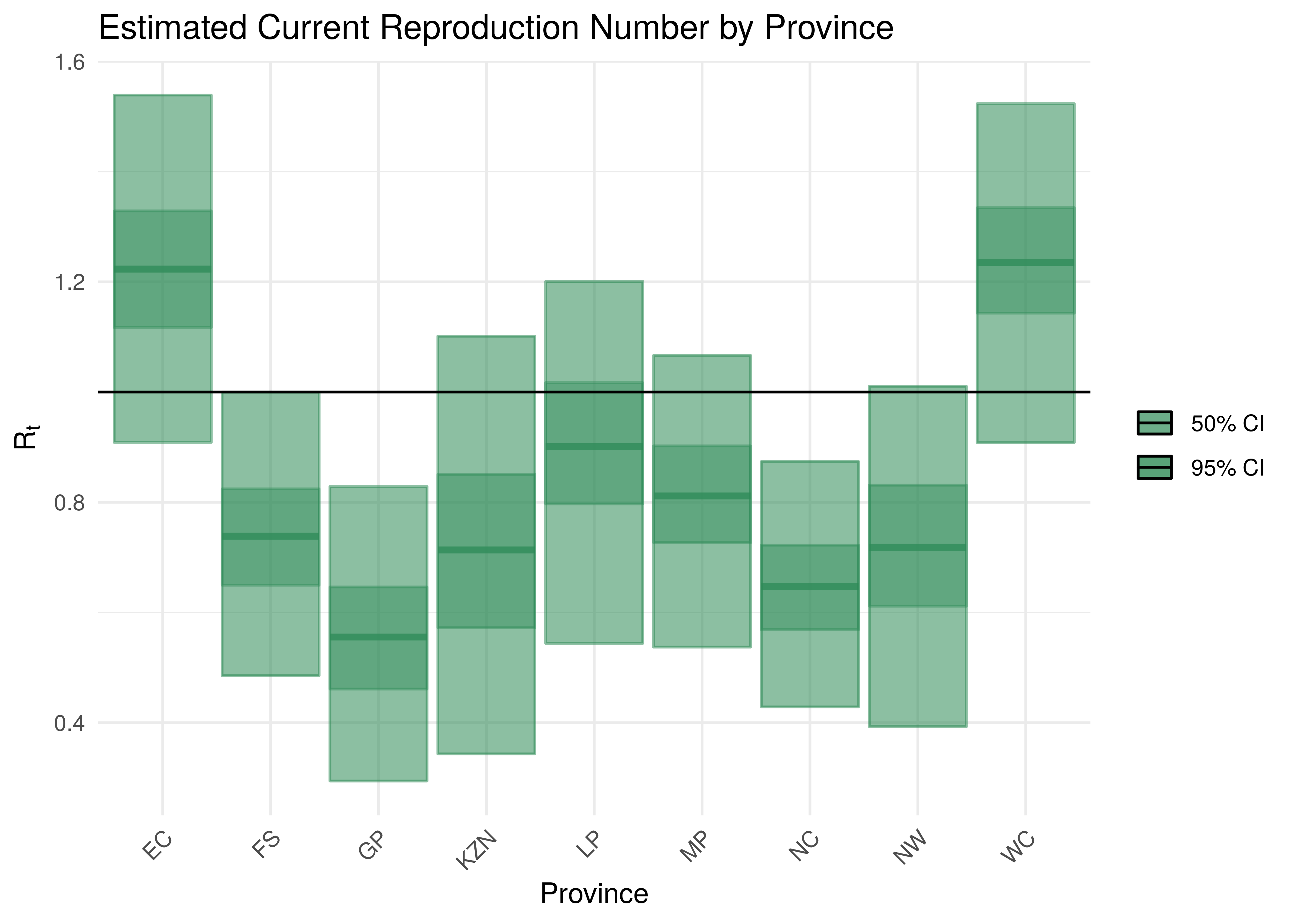
Current Reproduction Number by Province
8 Attack Rate and Cumulative Deaths as at 17 July 2021
The estimated attack rate and cumulative deaths (with 95% confidence intervals) are tabulated below (as at 17 July 2021).
The attack rate is the proportion of the population infected to date. This figure has to be estimated, because many that are infected experience no or mild symptoms, thus they may not seek medical advice and hence will never be tested.
Cumulative deaths are also inexact due to the fact that it’s based off an uncertain proportion of excess deaths which also needs to be projected to the latest date.
The confidence intervals for these estimates remain wide.
| Province | Attack Rate | Cumulative Deaths |
|---|---|---|
| EC | 64.8% [50.4%-75.9%] | 31 094 [ 25 216 - 37 880] |
| FS | 75.1% [57.4%-87.6%] | 10 955 [ 8 883 - 13 108] |
| GP | 80.0% [57.4%-93.3%] | 40 815 [ 31 875 - 51 178] |
| KZN | 65.4% [50.1%-77.6%] | 34 601 [ 27 761 - 42 355] |
| LP | 74.7% [52.0%-89.7%] | 18 754 [ 14 529 - 23 760] |
| MP | 76.3% [57.4%-89.2%] | 13 643 [ 10 869 - 16 721] |
| NC | 80.9% [66.3%-89.9%] | 5 850 [ 4 848 - 7 031] |
| NW | 73.6% [48.2%-90.8%] | 11 156 [ 8 473 - 14 342] |
| WC | 64.7% [45.9%-82.8%] | 17 403 [ 13 792 - 21 619] |
| South Africa | 72.2% [60.7%-80.7%] | 184 271 [166 917 - 203 239] |
9 Projections
One of the reasons we build models is so that we can make sense of the future or indeed the past. We can project forward models to assess the impact of varying assumptions on future outcomes. This gives us a sense of how changes in actions may impact the future. I.e. it allows us to answer “what if” questions. Note however that in projecting the future we are extrapolating, and due care needs to be taken. There are numerous limitations to this model and these projections dicussed below but the author is also of the opinion that the projections add value in that they indicate a significant range across the scenarios projected and in such a manner inform discussion.
All models are wrong but some are useful - George Box [14]
An incorrect model can be useful because it enables a better understanding of the model and the phenomena being modelled.
Note detailed projection output can be found here.
Projections are done using constant, increasing and decreasing mobility but other interventions are left constant. It should also be noted that the \(\epsilon_{w_m(t),m}\) are projected forward at constant levels and are not adjusted for projection purposes.
The \(\epsilon_{w_m(t),m}\) is held at “current” levels when projecting forwards. It should be noted that these levels are set 28 days prior as recent deaths only affect infections that occurred prior to that. Based on the observed calibration for Western Cape there is a possibility that this may be resulting in too low recent infections.
9.1 No change in Mobility
In this projection mobility is held constant at current levels. Level 4 interventions are left intact. It is also assumed that the AR(2) term remains at current levels.
The result of this scenario as at 30 September 2021 and 31 December 2021 are tabulated below. Note based on these it would appear that some provinces have already reached the peak in daily deaths.
| Province | Attack Rate | Deaths | Peak Daily Deaths | Peak Date |
|---|---|---|---|---|
| EC | 77.2% [59.7%-89.4%] | 37 838 [ 29 183- 49 371] | 302 | 2020-12-30 |
| FS | 77.7% [60.5%-88.8%] | 11 997 [ 9 670- 14 737] | 74 | 2020-08-05 |
| GP | 82.7% [61.8%-93.8%] | 50 731 [ 38 769- 65 633] | 510 | 2021-07-12 |
| KZN | 66.7% [50.8%-80.4%] | 35 539 [ 28 192- 44 526] | 502 | 2021-01-12 |
| LP | 84.2% [67.2%-93.0%] | 26 736 [ 20 456- 35 038] | 268 | 2021-01-19 |
| MP | 82.1% [65.3%-91.4%] | 16 995 [ 13 317- 21 562] | 159 | 2021-01-20 |
| NC | 82.0% [68.6%-90.1%] | 6 138 [ 5 136- 7 376] | 36 | 2021-05-29 |
| NW | 78.9% [54.6%-91.9%] | 14 601 [ 10 587- 19 502] | 118 | 2021-07-18 |
| WC | 83.5% [63.9%-93.1%] | 27 938 [ 20 347- 37 054] | 237 | 2021-08-08 |
| South Africa | 78.7% [69.1%-85.7%] | 228 512 [202 793-265 383] | 1 680 | 2021-01-14 |
| Province | Attack Rate | Deaths | Peak Daily Deaths | Peak Date |
|---|---|---|---|---|
| EC | 78.7% [62.3%-89.4%] | 39 657 [ 30 362- 51 257] | 302 | 2020-12-30 |
| FS | 77.8% [60.7%-88.8%] | 12 040 [ 9 710- 14 871] | 74 | 2020-08-05 |
| GP | 82.7% [61.9%-93.8%] | 50 775 [ 38 914- 65 636] | 510 | 2021-07-12 |
| KZN | 66.9% [50.8%-80.8%] | 35 760 [ 28 232- 45 225] | 502 | 2021-01-12 |
| LP | 84.2% [67.7%-93.0%] | 26 871 [ 20 638- 35 293] | 268 | 2021-01-19 |
| MP | 82.2% [65.4%-91.4%] | 17 066 [ 13 405- 21 635] | 159 | 2021-01-20 |
| NC | 82.1% [68.6%-90.1%] | 6 145 [ 5 142- 7 395] | 36 | 2021-05-29 |
| NW | 78.9% [55.0%-91.9%] | 14 654 [ 10 690- 19 535] | 118 | 2021-07-18 |
| WC | 83.7% [66.0%-93.1%] | 28 337 [ 21 139- 37 298] | 237 | 2021-08-08 |
| South Africa | 78.9% [69.6%-85.9%] | 231 305 [205 129-269 433] | 1 680 | 2021-01-14 |
9.2 Increase in mobility
This scenario assumes future mobility increases by a fixed value of 0.1. Other interventions are left intact. It is also assumed that the AR(2) term remains at current levels.
The attack rate and deaths after increasing mobility are tabulated below (as at 30 September 2021 and 31 December 2021).
| Province | Attack Rate | Deaths | Peak Daily Deaths | Peak Date |
|---|---|---|---|---|
| EC | 78.9% [61.3%-90.2%] | 38 567 [ 29 620- 50 386] | 302 | 2020-12-30 |
| FS | 78.2% [61.2%-88.9%] | 12 061 [ 9 728- 14 904] | 74 | 2020-08-05 |
| GP | 83.1% [62.6%-93.8%] | 50 975 [ 39 080- 65 876] | 510 | 2021-07-12 |
| KZN | 67.1% [51.0%-81.1%] | 35 669 [ 28 227- 44 872] | 502 | 2021-01-12 |
| LP | 85.1% [70.0%-93.2%] | 27 043 [ 20 727- 35 461] | 268 | 2021-01-19 |
| MP | 82.9% [66.5%-91.6%] | 17 137 [ 13 465- 21 722] | 159 | 2021-01-20 |
| NC | 82.2% [68.9%-90.1%] | 6 149 [ 5 145- 7 403] | 36 | 2021-05-29 |
| NW | 79.8% [56.3%-92.0%] | 14 764 [ 10 778- 19 685] | 118 | 2021-07-18 |
| WC | 85.1% [68.3%-93.5%] | 28 491 [ 20 954- 37 609] | 246 | 2021-08-10 |
| South Africa | 79.5% [70.4%-86.2%] | 230 855 [204 714-269 250] | 1 680 | 2021-01-14 |
Based on the above an increase mobility could mean roughly 2 000 more deaths by end of September 2021.
| Province | Attack Rate | Deaths | Peak Daily Deaths | Peak Date |
|---|---|---|---|---|
| EC | 80.6% [64.8%-90.3%] | 40 622 [ 31 213- 52 170] | 302 | 2020-12-30 |
| FS | 78.3% [61.3%-88.9%] | 12 125 [ 9 794- 15 029] | 74 | 2020-08-05 |
| GP | 83.1% [62.8%-93.8%] | 51 043 [ 39 269- 65 933] | 510 | 2021-07-12 |
| KZN | 67.4% [51.1%-81.7%] | 36 019 [ 28 302- 45 962] | 502 | 2021-01-12 |
| LP | 85.2% [70.8%-93.2%] | 27 203 [ 20 936- 35 654] | 268 | 2021-01-19 |
| MP | 83.0% [67.3%-91.6%] | 17 230 [ 13 602- 21 786] | 159 | 2021-01-20 |
| NC | 82.2% [69.1%-90.1%] | 6 159 [ 5 154- 7 423] | 36 | 2021-05-29 |
| NW | 79.9% [57.1%-92.0%] | 14 843 [ 10 890- 19 740] | 118 | 2021-07-18 |
| WC | 85.4% [70.4%-93.5%] | 28 902 [ 21 990- 37 947] | 246 | 2021-08-10 |
| South Africa | 79.8% [70.9%-86.4%] | 234 146 [207 447-274 431] | 1 680 | 2021-01-14 |
Based on the above an increase mobility could mean roughly 3 000 more deaths by the end of December 2021.
9.3 Decreased mobility
This scenario assumes future mobility decreases by a fixed value of 0.1. It is also assumed that the AR(2) term remains at current levels.
The attack rate and deaths after decreased mobility are tabulated below (as at 30 September 2021 and 31 December 2021).
| Province | Attack Rate | Deaths | Peak Daily Deaths | Peak Date |
|---|---|---|---|---|
| EC | 75.5% [58.0%-88.5%] | 37 142 [ 28 759- 48 348] | 302 | 2020-12-30 |
| FS | 77.3% [59.7%-88.7%] | 11 942 [ 9 622- 14 614] | 74 | 2020-08-05 |
| GP | 82.3% [61.3%-93.8%] | 50 518 [ 38 545- 65 375] | 510 | 2021-07-12 |
| KZN | 66.5% [50.7%-79.8%] | 35 437 [ 28 154- 44 330] | 502 | 2021-01-12 |
| LP | 83.2% [64.4%-92.8%] | 26 435 [ 20 118- 34 709] | 268 | 2021-01-19 |
| MP | 81.5% [63.6%-91.3%] | 16 863 [ 13 221- 21 395] | 159 | 2021-01-20 |
| NC | 81.9% [68.3%-90.1%] | 6 129 [ 5 120- 7 359] | 36 | 2021-05-29 |
| NW | 78.1% [53.4%-91.8%] | 14 459 [ 10 463- 19 325] | 118 | 2021-07-18 |
| WC | 81.7% [60.0%-92.6%] | 27 360 [ 19 657- 36 494] | 228 | 2021-08-07 |
| South Africa | 77.9% [67.6%-85.3%] | 226 284 [200 620-262 166] | 1 680 | 2021-01-14 |
Based on the above a decrease in mobility could mean roughly 2 000 fewer deaths by end of September 2021.
| Province | Attack Rate | Deaths | Peak Daily Deaths | Peak Date |
|---|---|---|---|---|
| EC | 76.8% [59.5%-88.5%] | 38 664 [ 29 561- 50 265] | 302 | 2020-12-30 |
| FS | 77.4% [59.8%-88.7%] | 11 971 [ 9 642- 14 680] | 74 | 2020-08-05 |
| GP | 82.3% [61.3%-93.8%] | 50 547 [ 38 568- 65 376] | 510 | 2021-07-12 |
| KZN | 66.6% [50.7%-80.3%] | 35 581 [ 28 173- 44 695] | 502 | 2021-01-12 |
| LP | 83.3% [64.7%-92.8%] | 26 542 [ 20 276- 34 753] | 268 | 2021-01-19 |
| MP | 81.5% [63.8%-91.3%] | 16 916 [ 13 308- 21 508] | 159 | 2021-01-20 |
| NC | 81.9% [68.3%-90.1%] | 6 133 [ 5 122- 7 375] | 36 | 2021-05-29 |
| NW | 78.1% [53.5%-91.8%] | 14 494 [ 10 542- 19 344] | 118 | 2021-07-18 |
| WC | 82.0% [61.3%-92.6%] | 27 720 [ 20 314- 36 614] | 228 | 2021-08-07 |
| South Africa | 78.1% [68.1%-85.4%] | 228 568 [202 687-265 818] | 1 680 | 2021-01-14 |
Based on the above a decrease in mobility could mean roughly 3 000 fewer deaths by the end of December 2021.
9.4 Worst Case Scenario
This scenario assumes future mobility increases by a fixed value of 0.1, mask wearing is eliminated. It is also assumed that the AR(2) term remains at current levels.
The attack rate and deaths are tabulated below (as at 30 September 2021 and 31 December 2021). This would be a relatively extreme worst case scenario as this essentially assumes not mitigation measures in place and would probably be close to the absolute worst case.
| Province | Attack Rate | Deaths | Peak Daily Deaths | Peak Date |
|---|---|---|---|---|
| EC | 86.0% [70.4%-94.2%] | 42 005 [ 31 834- 55 768] | 302 | 2020-12-30 |
| FS | 81.7% [66.7%-90.5%] | 12 530 [ 10 097- 15 992] | 74 | 2020-08-05 |
| GP | 85.9% [72.0%-93.9%] | 52 683 [ 41 344- 68 032] | 510 | 2021-07-12 |
| KZN | 70.8% [53.0%-87.5%] | 36 969 [ 28 758- 48 209] | 502 | 2021-01-12 |
| LP | 89.2% [80.4%-94.4%] | 28 401 [ 21 810- 37 671] | 268 | 2021-01-19 |
| MP | 86.6% [75.5%-92.8%] | 17 900 [ 14 081- 23 155] | 159 | 2021-01-20 |
| NC | 83.4% [72.0%-90.3%] | 6 227 [ 5 201- 7 573] | 36 | 2021-05-29 |
| NW | 85.4% [70.3%-93.0%] | 15 800 [ 11 653- 21 378] | 118 | 2021-07-18 |
| WC | 90.7% [81.8%-96.1%] | 30 522 [ 23 292- 40 329] | 304 | 2021-08-14 |
| South Africa | 83.7% [75.9%-90.0%] | 243 038 [212 285-292 645] | 1 680 | 2021-01-14 |
Based on the above the worst case scenario could result in roughly 15 000 more deaths by the end of September 2021.
| Province | Attack Rate | Deaths | Peak Daily Deaths | Peak Date |
|---|---|---|---|---|
| EC | 87.3% [76.3%-94.2%] | 44 116 [ 34 831- 57 278] | 302 | 2020-12-30 |
| FS | 82.3% [68.3%-90.5%] | 12 786 [ 10 241- 16 443] | 74 | 2020-08-05 |
| GP | 86.1% [73.1%-93.9%] | 52 995 [ 41 631- 68 278] | 510 | 2021-07-12 |
| KZN | 73.5% [55.1%-88.1%] | 39 222 [ 29 567- 52 409] | 502 | 2021-01-12 |
| LP | 89.3% [80.9%-94.4%] | 28 563 [ 22 057- 37 790] | 268 | 2021-01-19 |
| MP | 86.8% [76.5%-92.8%] | 18 074 [ 14 252- 23 456] | 159 | 2021-01-20 |
| NC | 83.7% [72.8%-90.4%] | 6 278 [ 5 230- 7 685] | 36 | 2021-05-29 |
| NW | 85.6% [72.4%-93.0%] | 15 994 [ 11 980- 21 569] | 118 | 2021-07-18 |
| WC | 90.8% [82.5%-96.1%] | 30 785 [ 23 845- 40 505] | 304 | 2021-08-14 |
| South Africa | 84.5% [76.8%-90.5%] | 248 813 [216 532-302 506] | 1 680 | 2021-01-14 |
Based on the above the worst case scenario could result in roughly 18 000 more deaths by the end of December 2021.
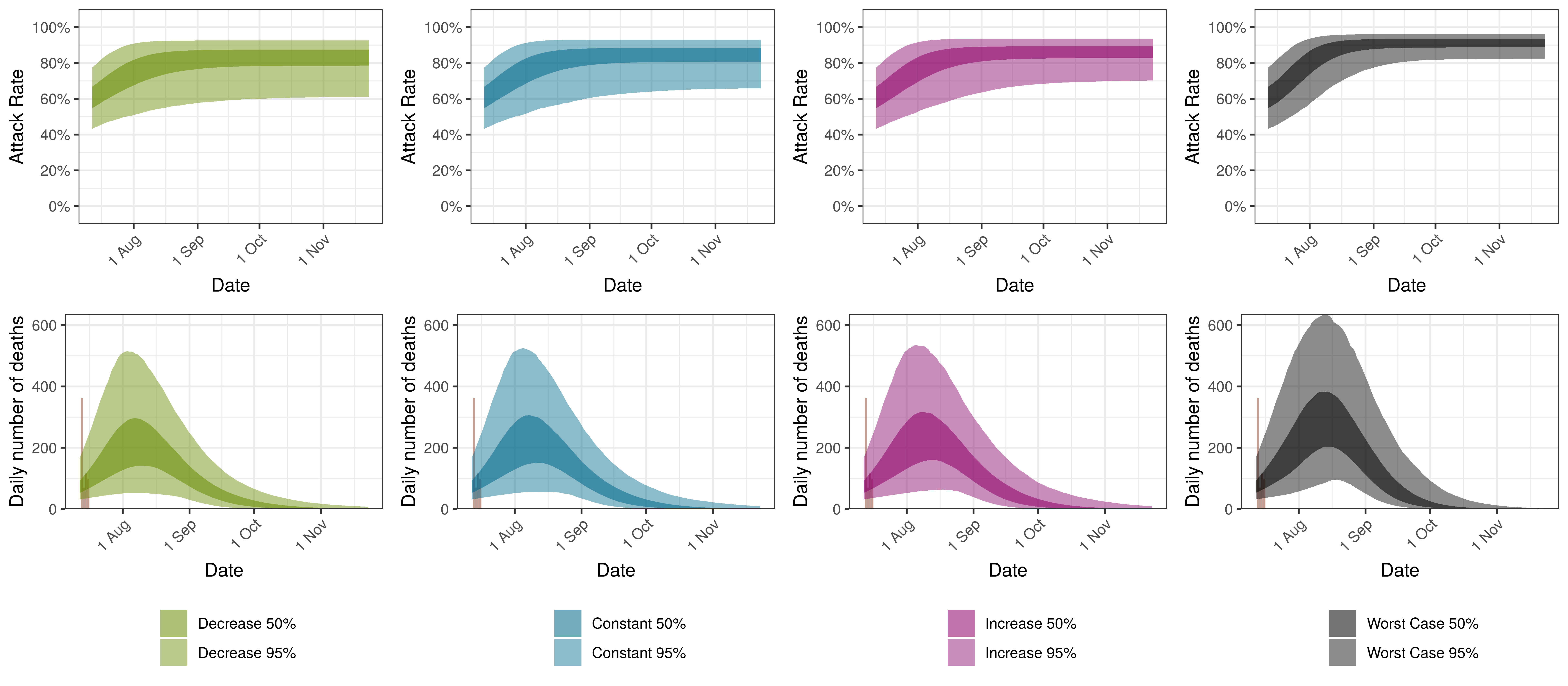
9.5 South Africa
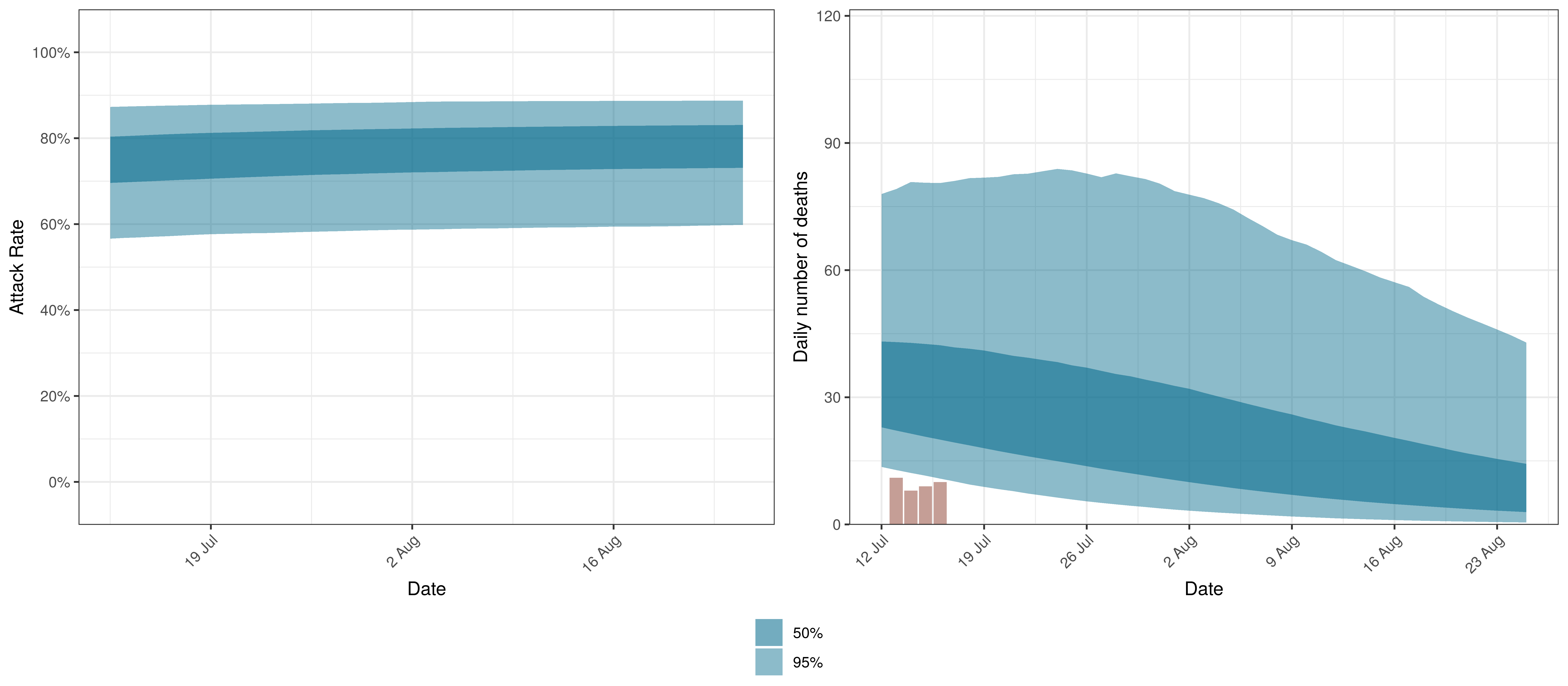
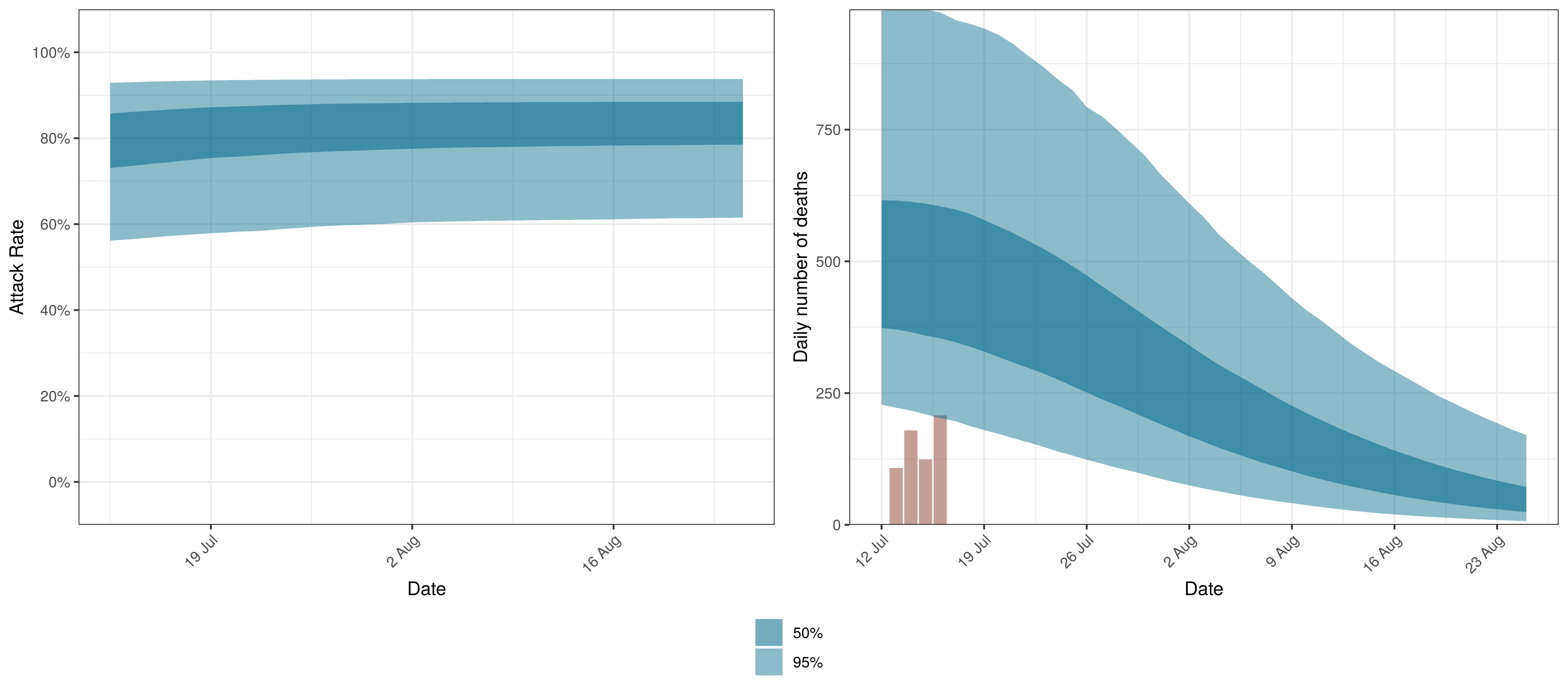
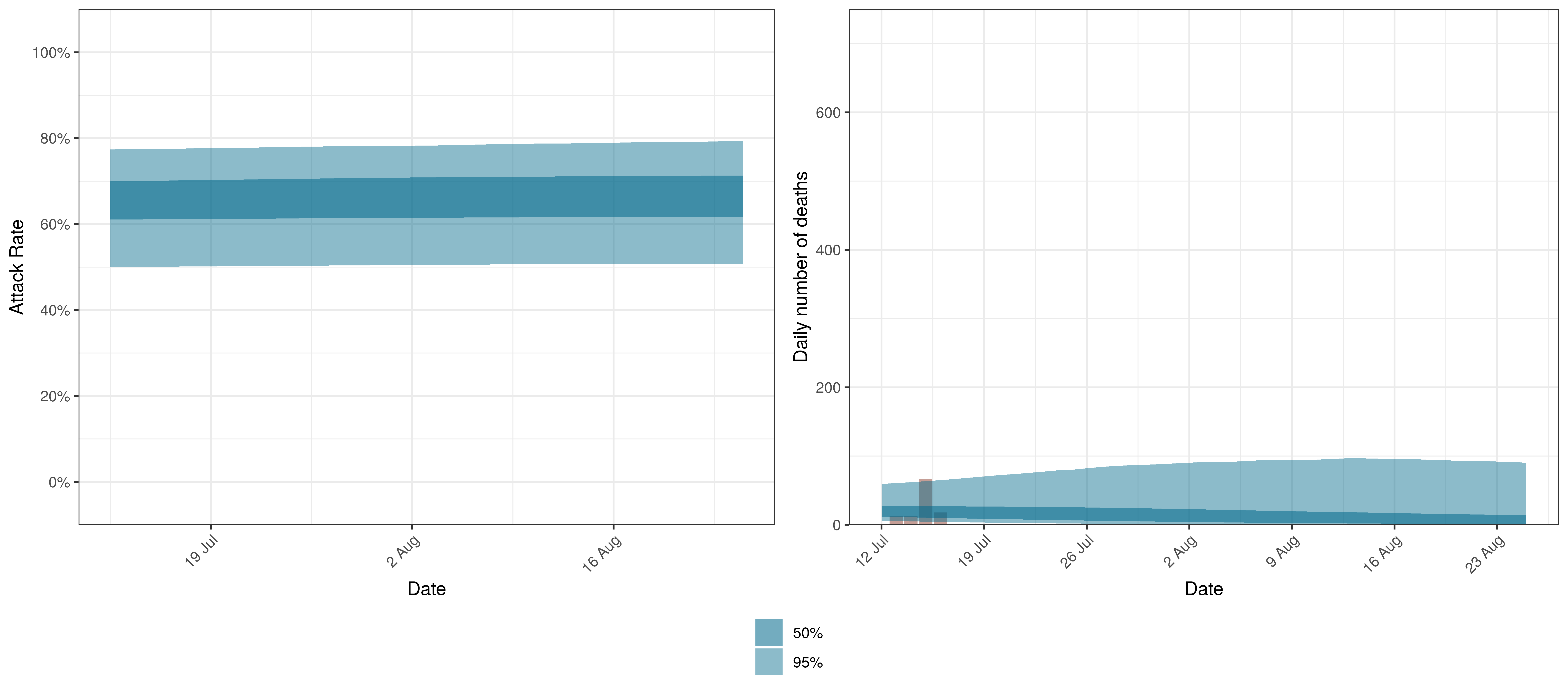
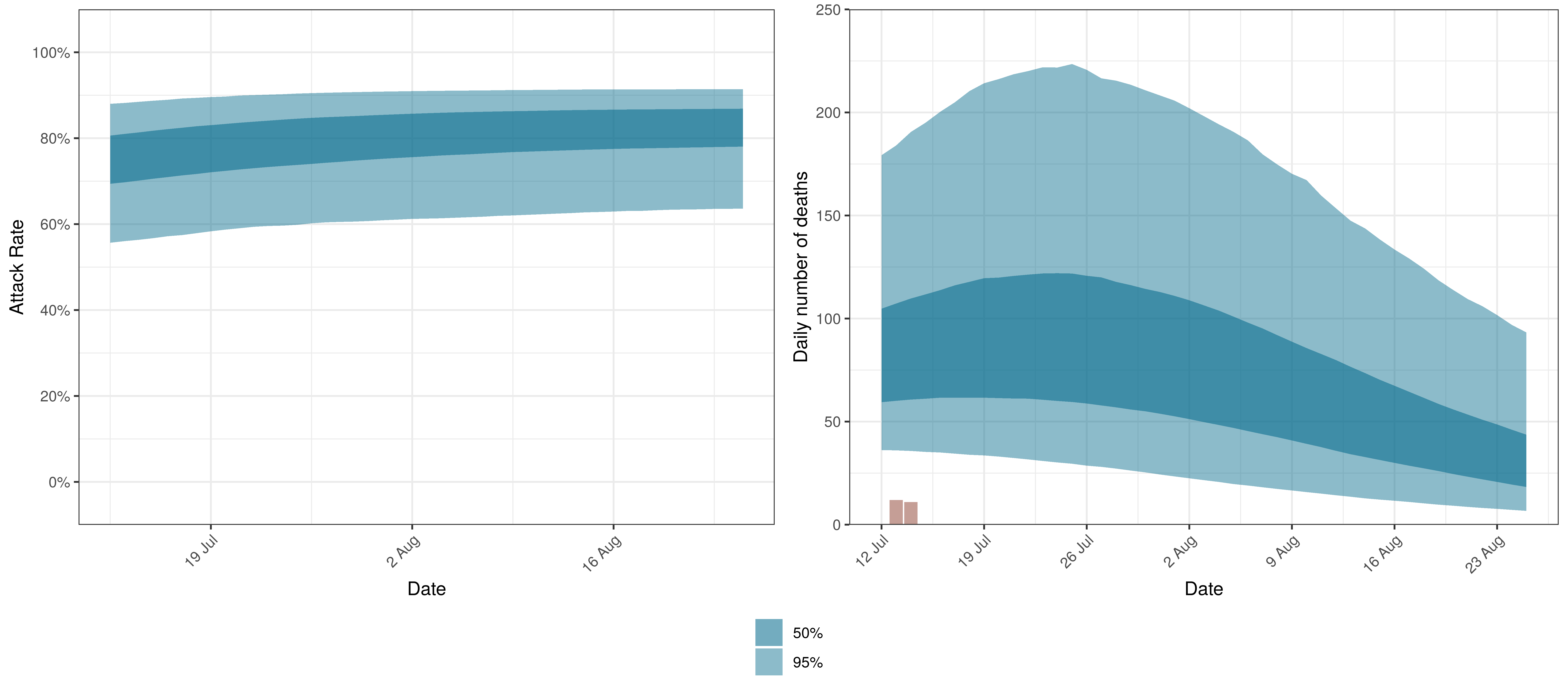
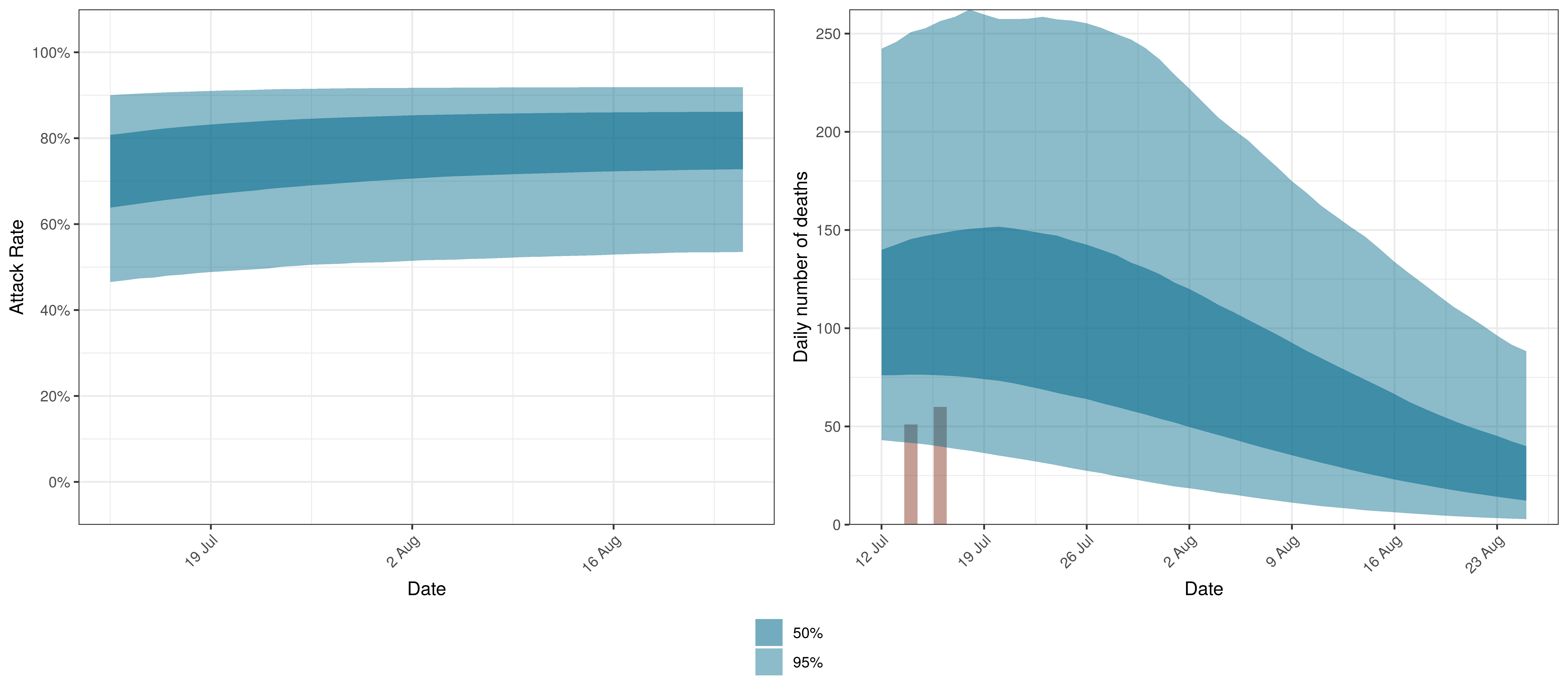
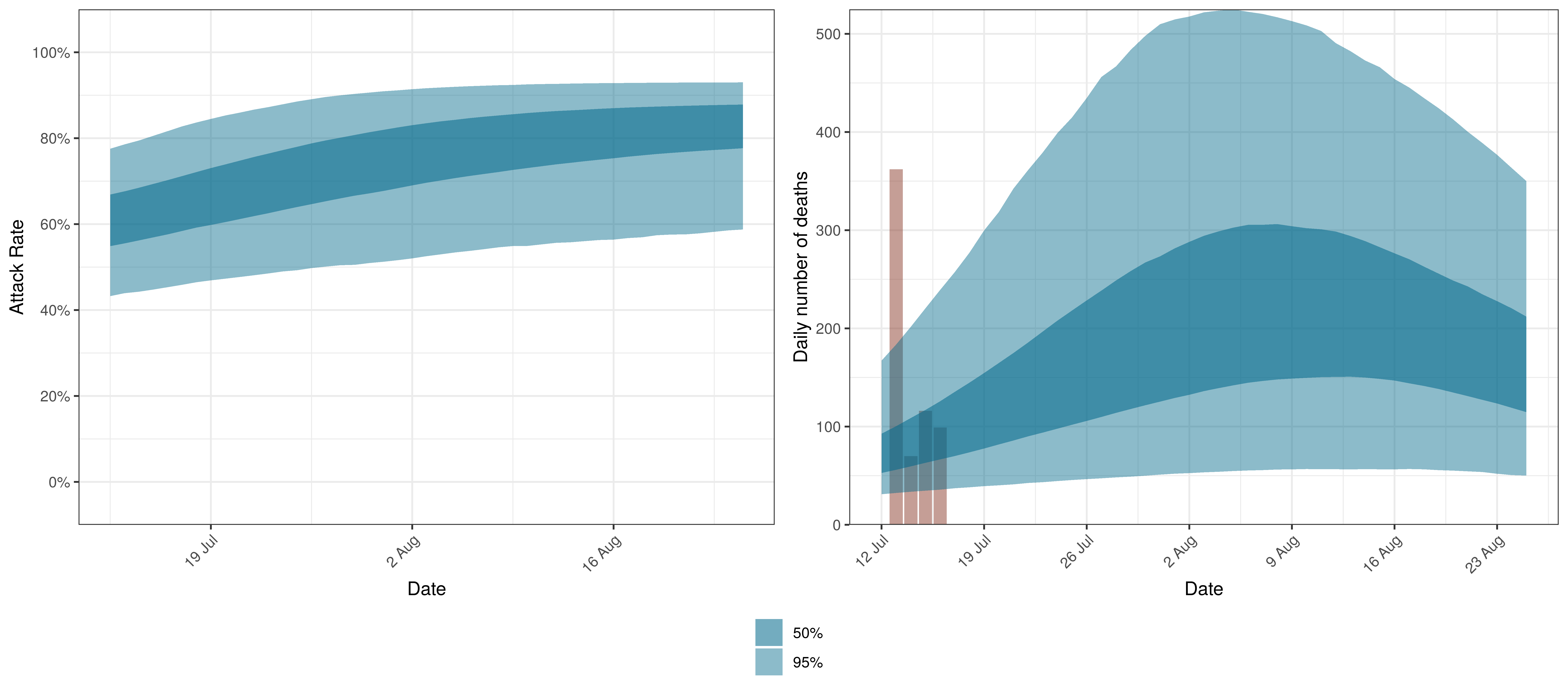
The results for South Africa as a whole are plotted below. This is the sum of the provincial projections.
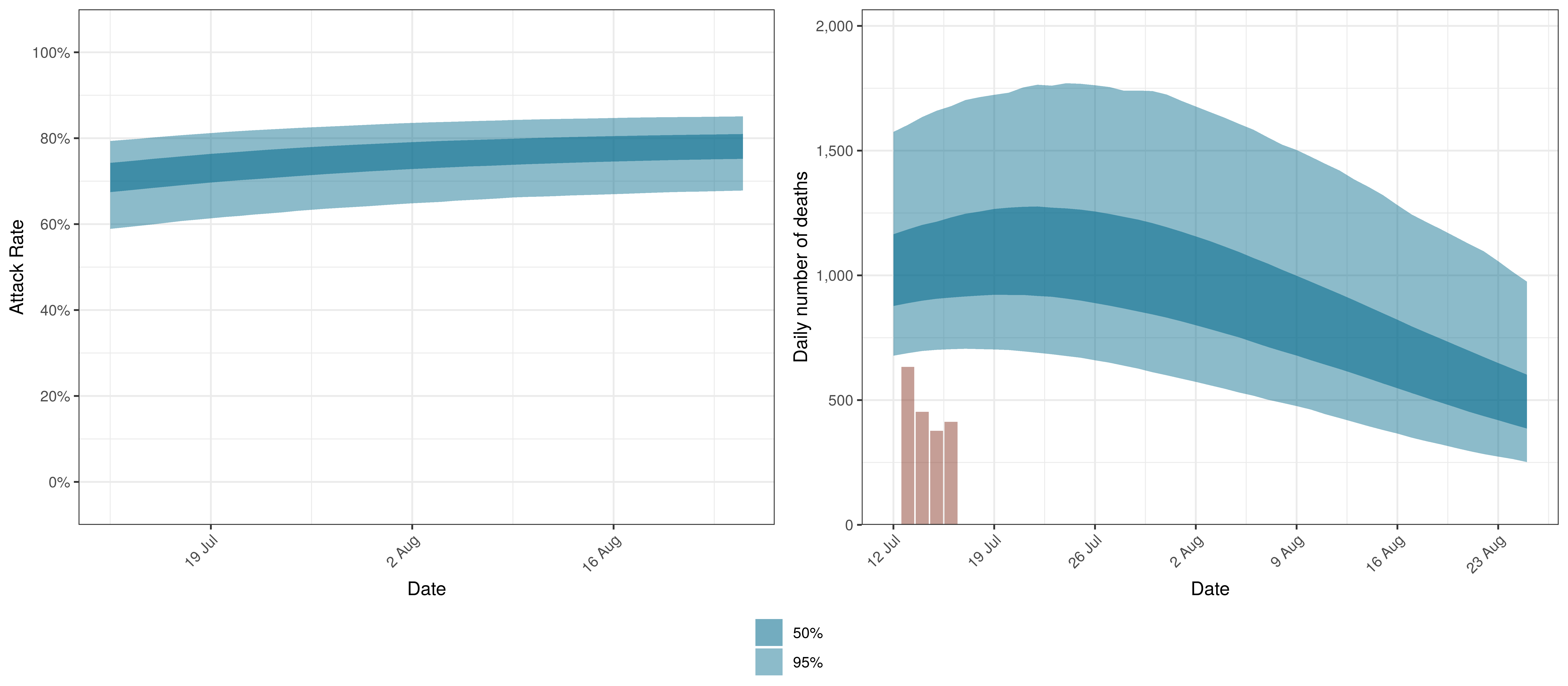
Projected Attack Rate and Daily Deaths in South Africa
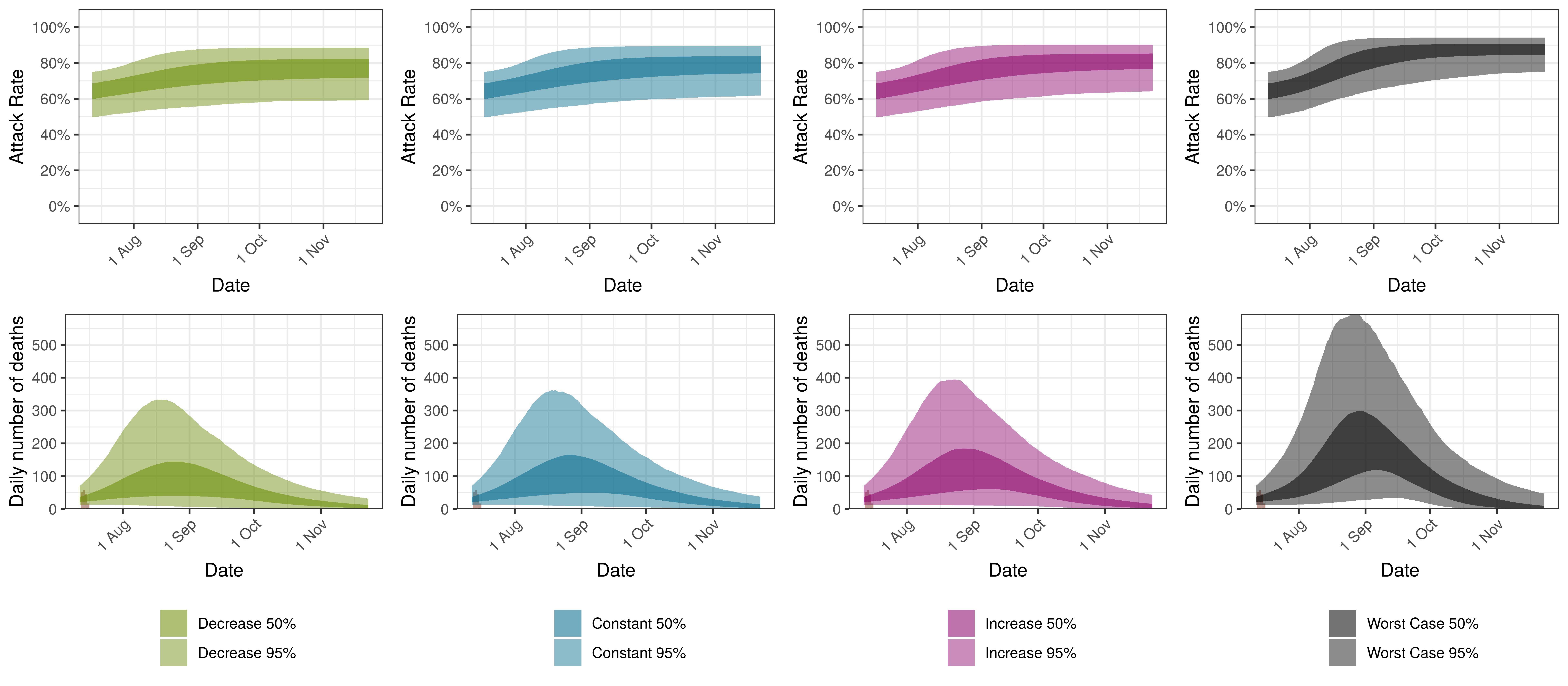
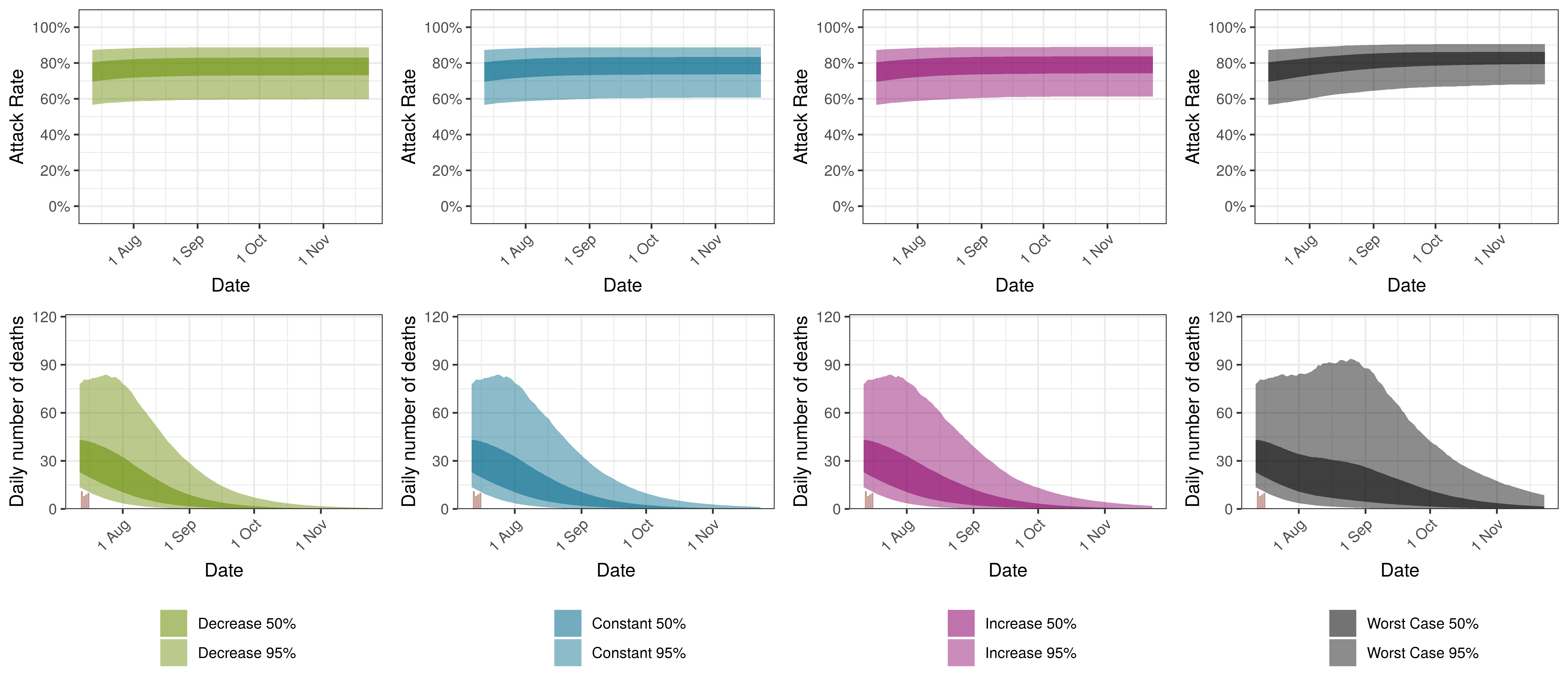
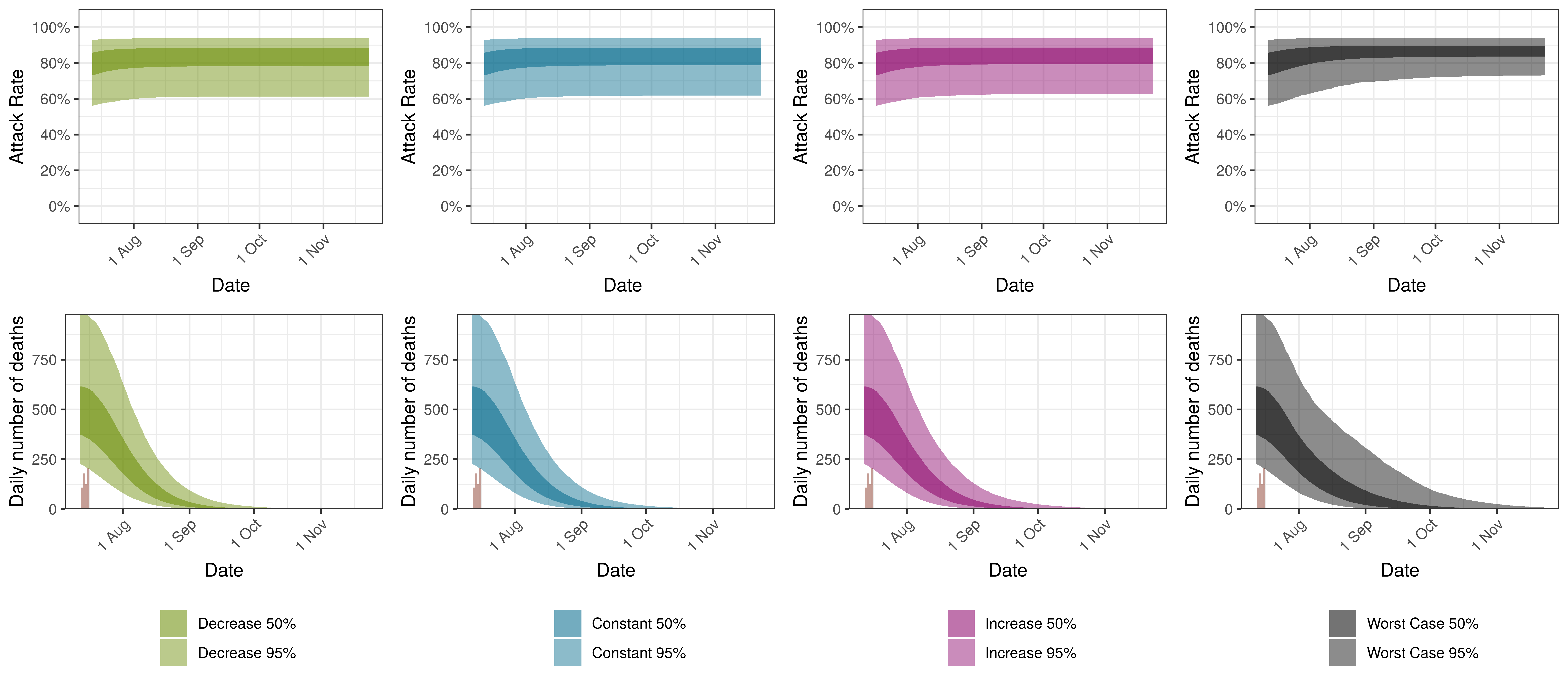
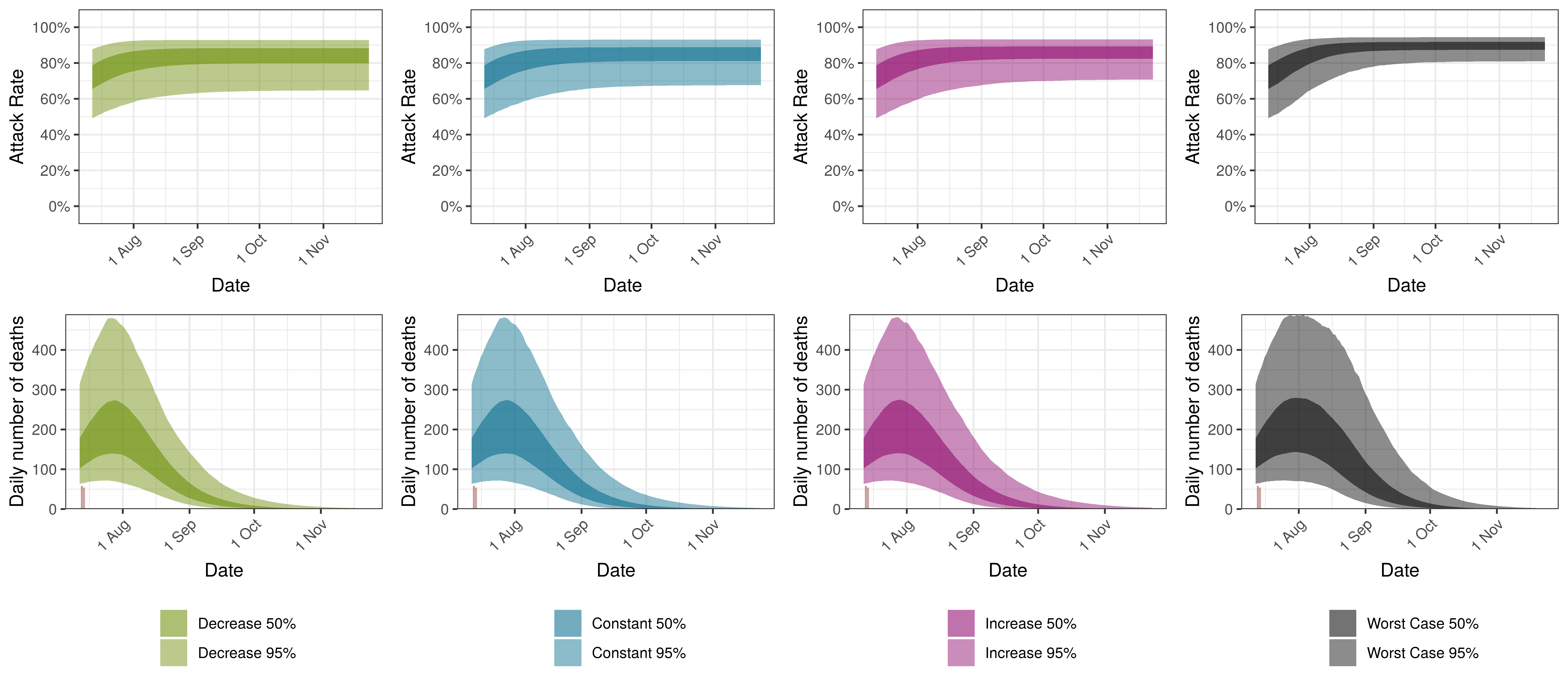
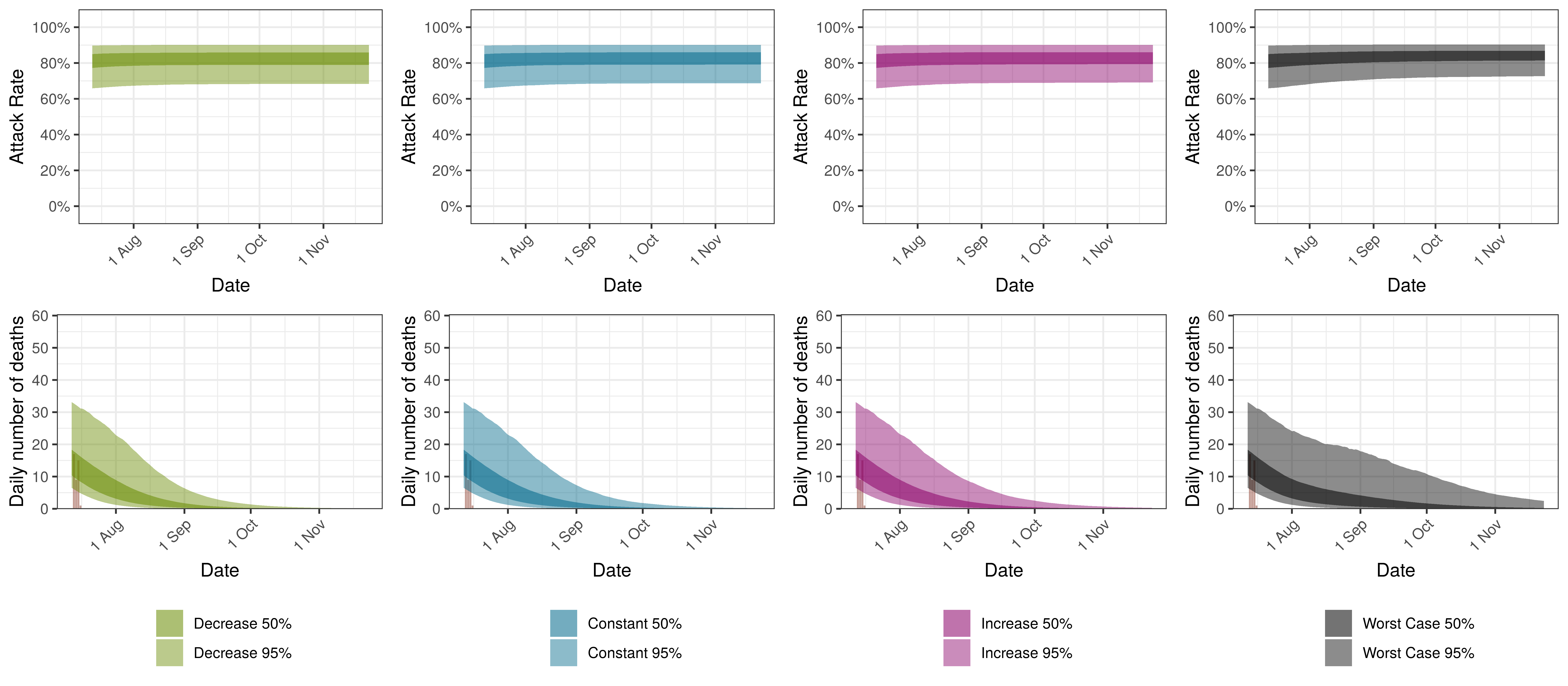
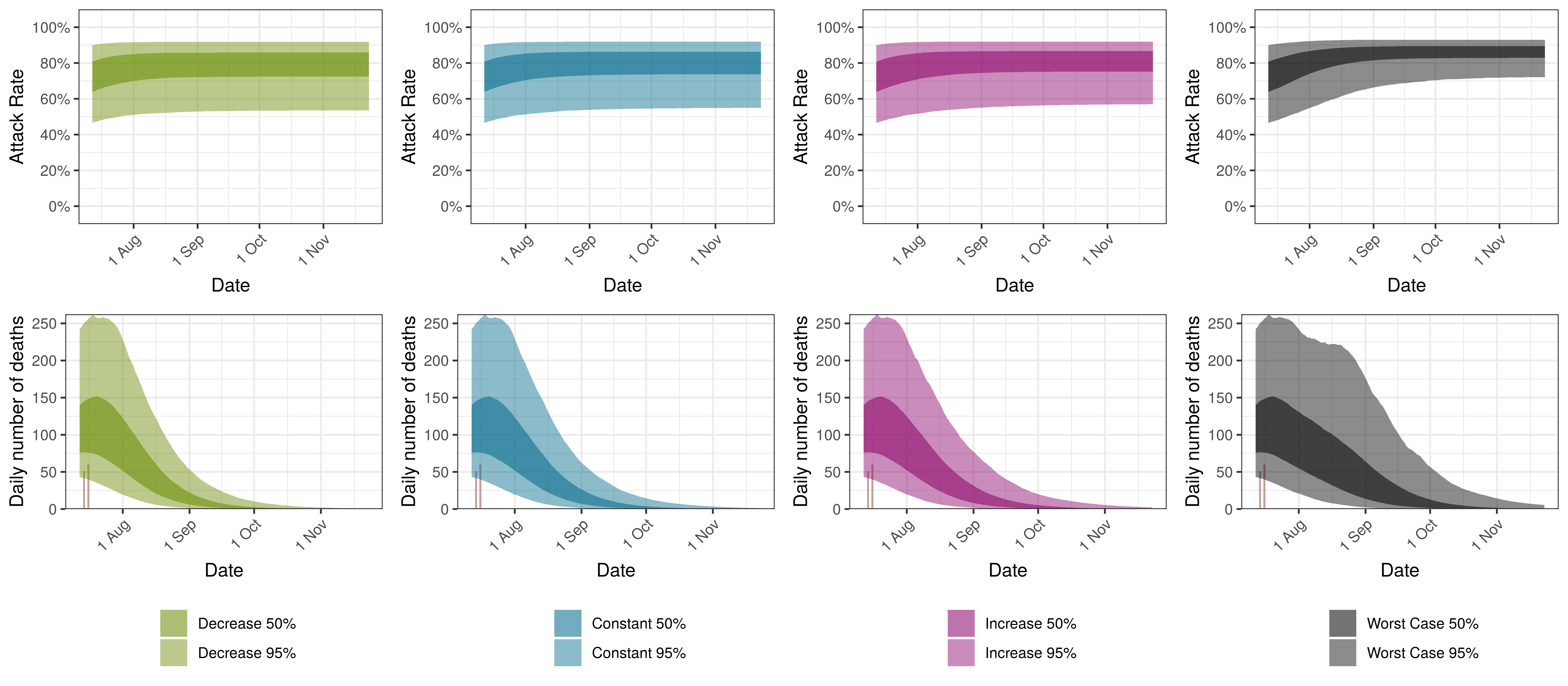
The attack rate and deaths over a longer period for the various scenarios are plotted below:
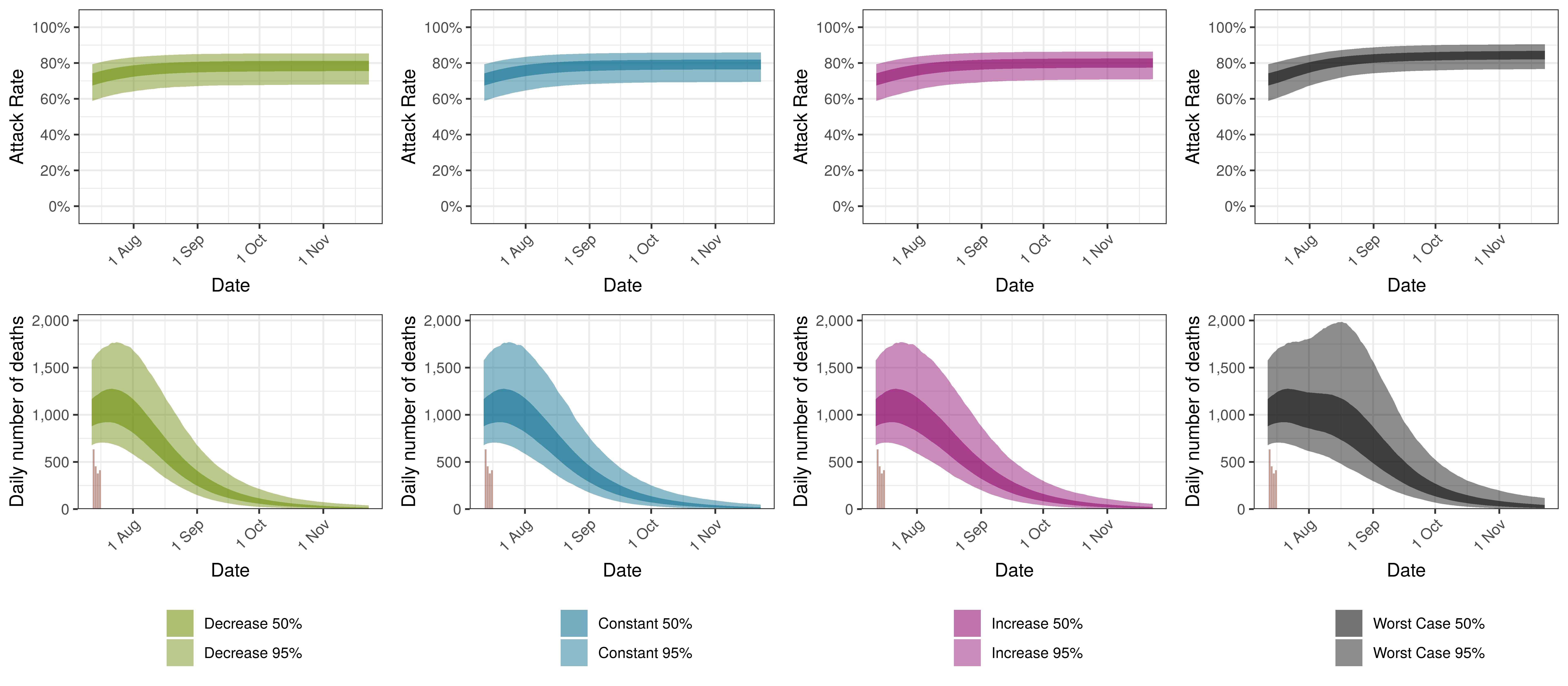
Projected Attack Rate and Daily Deaths in South Africa by Scenario
9.6 Eastern Cape
The projections for Eastern Cape are plotted below.
Projected Attack Rate and Daily Deaths in Eastern Cape
The attack rate and deaths over a longer period for the various scenarios are plotted below:
Projected Attack Rate and Daily Deaths in Eastern Cape by Scenario
9.7 Free State
The projections for the Free State are plotted below.
Projected Attack Rate and Daily Deaths in Free State
The attack rate and deaths over a longer period for the various scenarios are plotted below:
Projected Attack Rate and Daily Deaths in Free State by Scenario
9.8 Gauteng
The projections for Gauteng are plotted below.
Projected Attack Rate and Daily Deaths in Gauteng
The attack rate and deaths over a longer period for the various scenarios are plotted below:
Projected Attack Rate and Daily Deaths in Gauteng by Scenario
9.9 KwaZulu-Natal
The projections for KwaZulu-Natal are plotted below.
Projected Attack Rate and Daily Deaths in KwaZulu-Natal
The attack rate and deaths over a longer period for the various scenarios are plotted below:
Projected Attack Rate and Daily Deaths in KwaZulu-Natal by Scenario
9.10 Limpopo
The projections for Limpopo are plotted below.
Projected Attack Rate and Daily Deaths in Limpopo
The attack rate and deaths over a longer period for the various scenarios are plotted below:
Projected Attack Rate and Daily Deaths in Limpopo by Scenario
9.11 Mpumalanga
The projections for Mpumalanga are plotted below.
Projected Attack Rate and Daily Deaths in Mpumalanga
The attack rate and deaths over a longer period for the various scenarios are plotted below:
Projected Attack Rate and Daily Deaths in Mpumalanga by Scenario
9.12 Northern Cape
The projections for the Northern Cape are plotted below.
Projected Attack Rate and Daily Deaths in Northern Cape
The attack rate and deaths over a longer period for the various scenarios are plotted below:
Projected Attack Rate and Daily Deaths in Northern Cape by Scenario
9.13 North West
The projections for the North West are plotted below.
Projected Attack Rate and Daily Deaths in North West
The attack rate and deaths over a longer period for the various scenarios are plotted below:
Projected Attack Rate and Daily Deaths in North West by Scenario
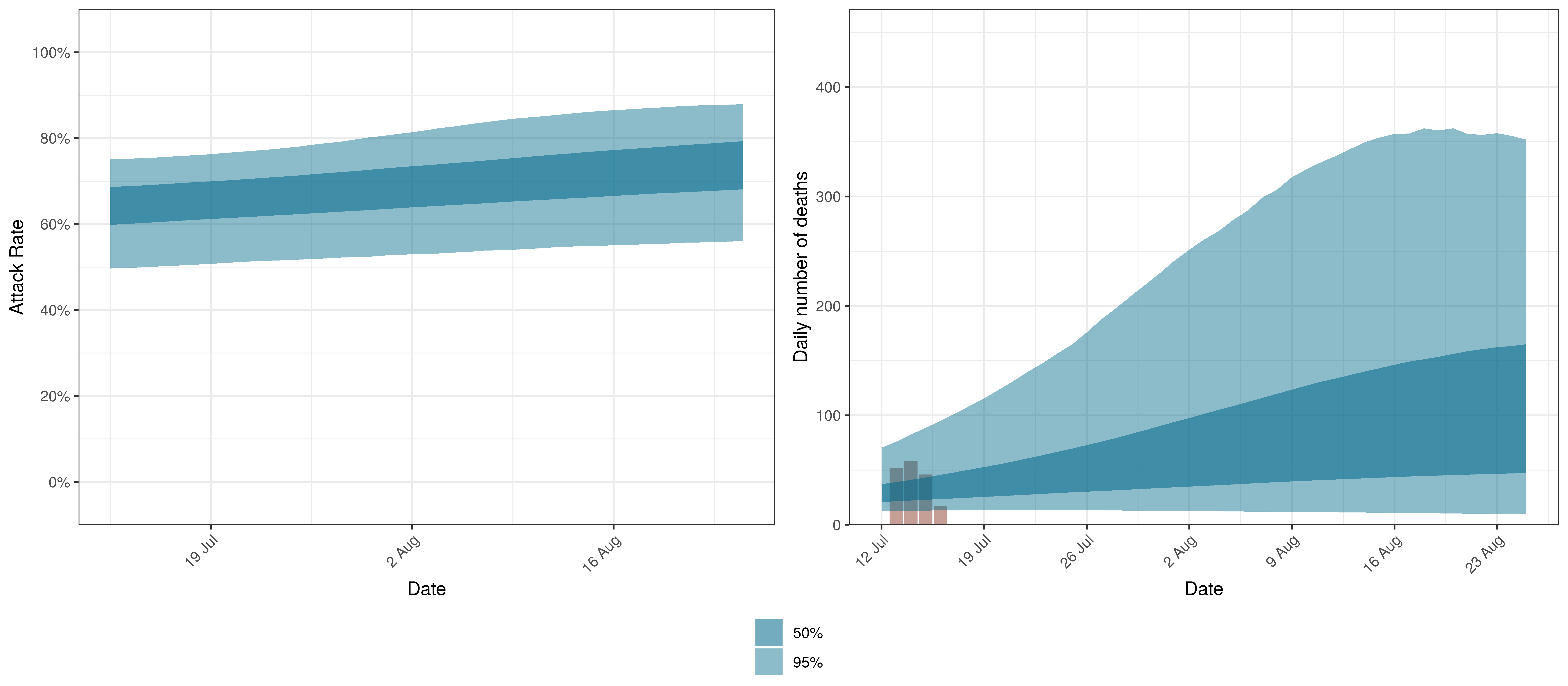
9.14 Western Cape
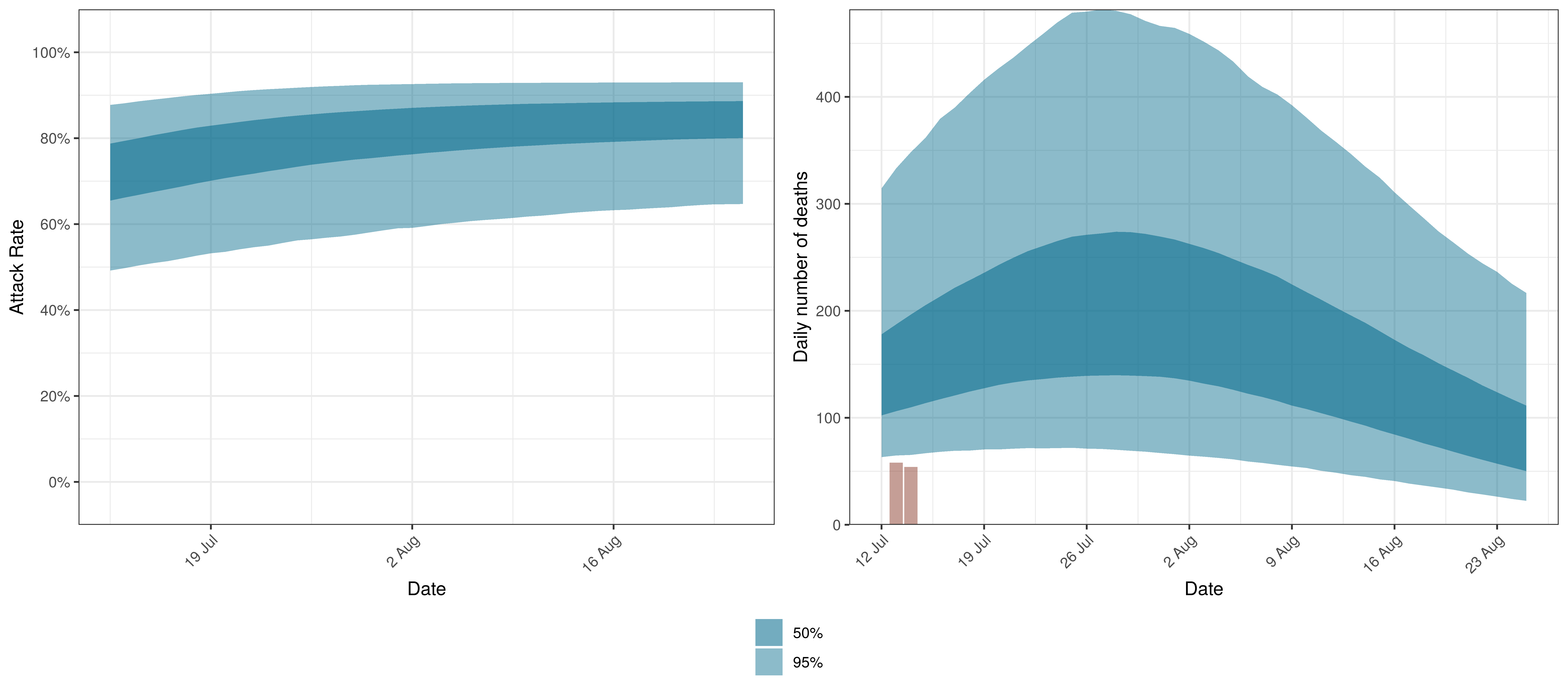
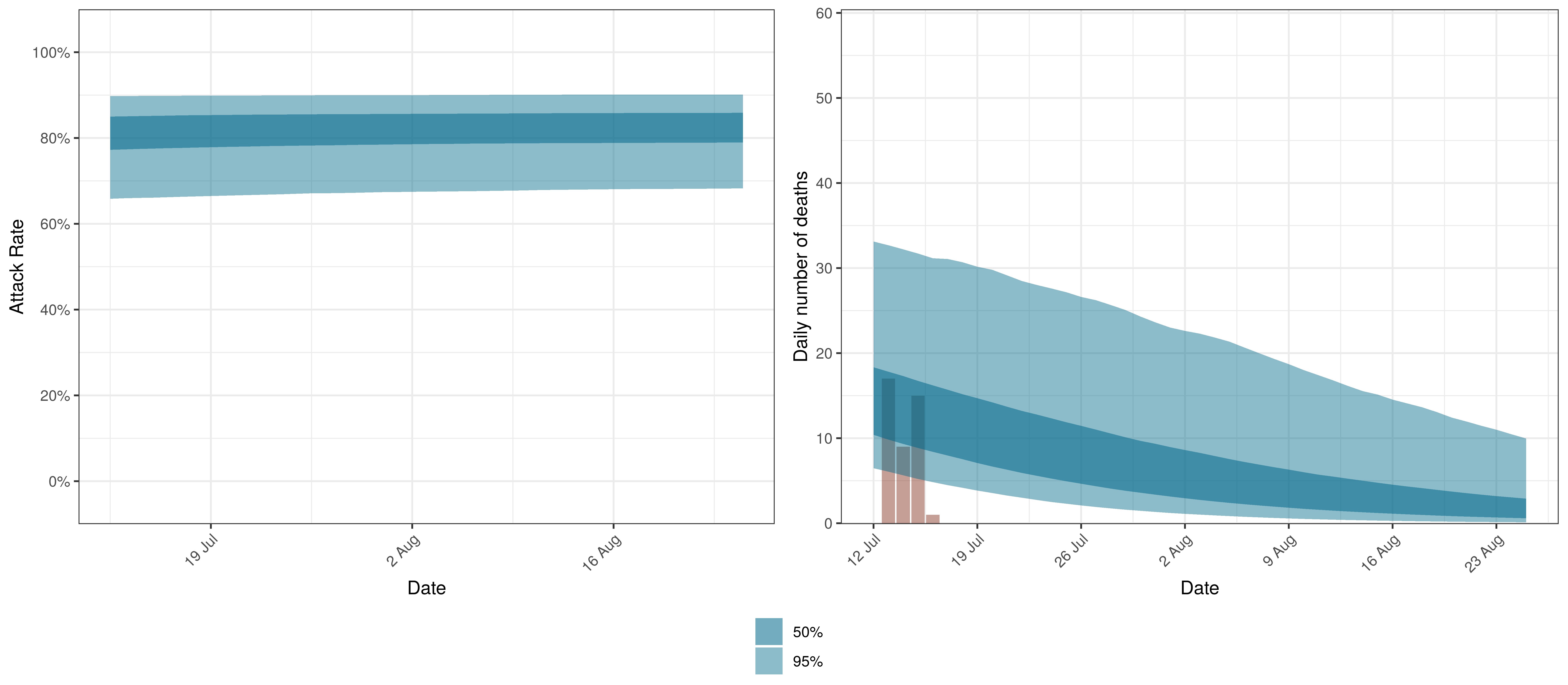
The projections for the Western Cape are plotted below.
Projected Attack Rate and Daily Deaths in Western Cape
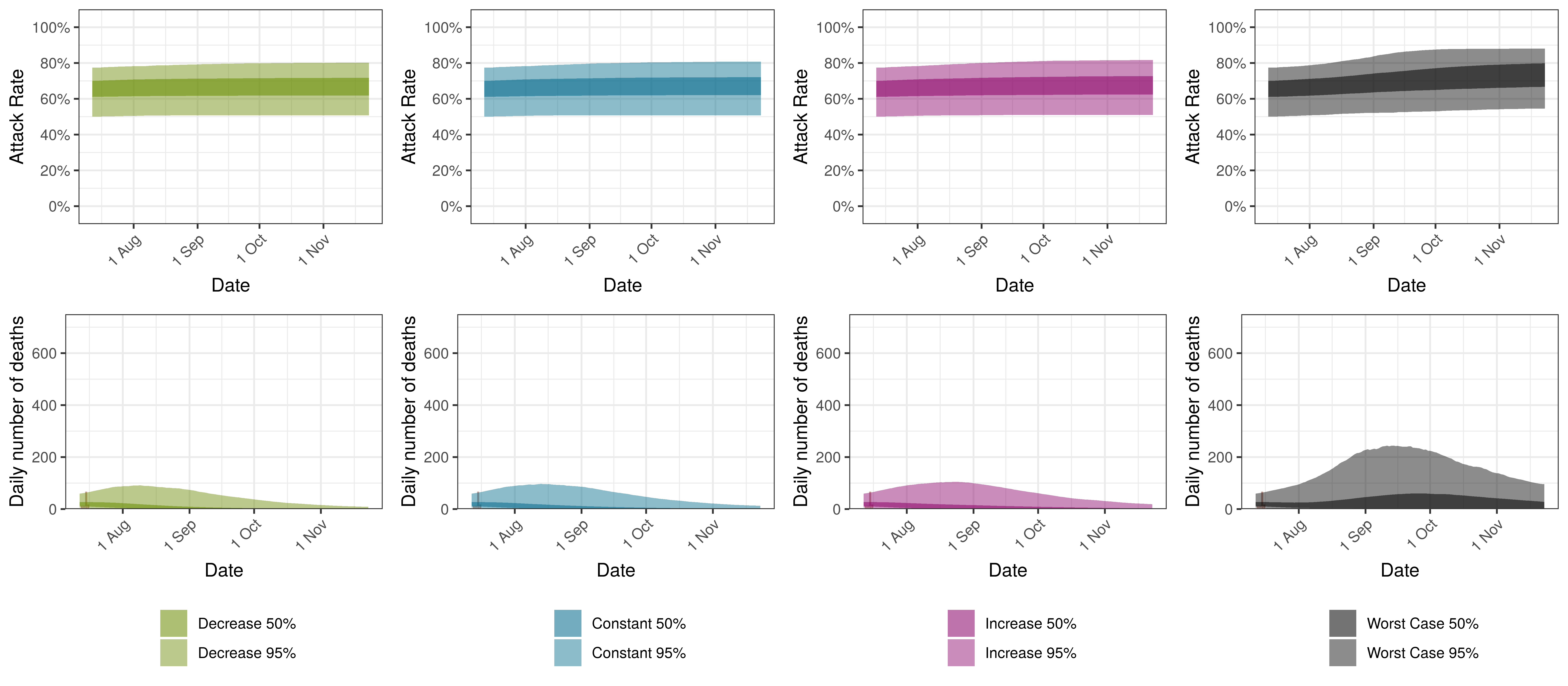
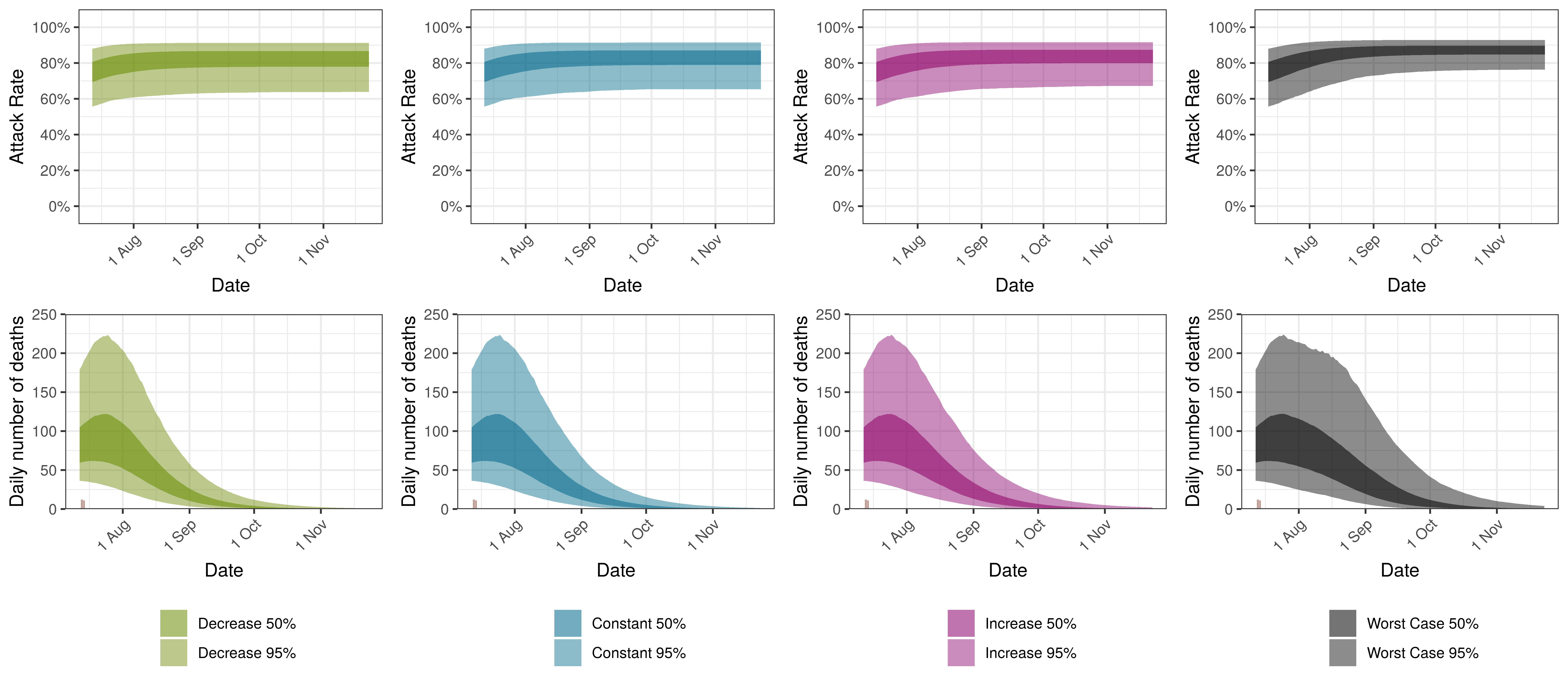
The attack rate and deaths over a longer period for the various scenarios are plotted below:
Projected Attack Rate and Daily Deaths in Western Cape by Scenario
10 Discussion
There remains significant uncertainty with all matters relating this epidemic. This includes uncertainty in data, assumptions and many epidemiological and medical matters relating to this disease. It is therefore likely that the model will not be accurate. It is also reflected in the wide confidence intervals of many of the results of the model.
Some researchers have gone as far as to say that it is not possible to accurately estimate the mean number of fatalities of pandemics based on data ([15] & [16]). This would indicate the goal of the paper may be futile.
This paper has however attempted to allow for uncertainty using the Bayesian approach here which results in at least some distribution of possible results, some of which are definitely catastrophic and some of which are less severe.
10.1 Limitations
This analysis has various limitations. A few are highlighted below but there are many. Perhaps the most important being the lack of good quality data.
- The model is based on somewhat limited data for South Africa. In particular the effects of lockdown in some of the provinces may be simple “extrapolations” using the fixed effect (\(\alpha\)) and shared prior of \(R_{0,m}\) from other provinces. As these fits are updated with new data though the model should be more accurate for each province resulting in better estimates.
- The model is a simplistic high-level single population model for each province. It contains no differentiation by age groups or any further details. This is required to make the hierarchical model manageable. It seems still to provide useful information on potential movements in the epidemic. However, this homogeneity may result in overestimation of attack rates and hence deaths.
- Similar to the above point various groups even of the same age may have varying susceptibility to the virus. Varying susceptibility may reduce the effective herd immunity threshold of the disease.
- The model does not take account of changes in many interventions that do not impact general mobility such as social distancing, handwashing and testing, tracing and isolation. The model does take account of the average impact of these interventions over time, but changes in these interventions will not be taken account of. It could be argued that the AR(2) autoregressive term is taking account of these factors.
- The paper does take account of mask-wearing, workplace screening and other NPIs introduced with the start of level 4 lockdown. This is done approximately and only measures the implementation of the regulation and not actual compliance with the regulations. These parameters may also not be capturing only this effect and may include other effects that occurred at the same time. Similarly these variable may not be fully capturing increased compliance with these regulations over time.
- Google Mobility data may not effectively cover the South African population. It is unclear how uniform the coverage is in say lower income populations who may have limited data and hence may not contribute significantly to the mobility indexes. Smartphone penetration in South Africa is estimated to exceed 90% [17] though. So the representative nature may be driven mainly by access to data as well as how many people have enabled the feature used to generate the data (Location History). Changes in mobility may have a different impact on various segments of the population.
- IFR assumptions may be wrong:
- It is based on Chinese data and may therefore be higher or lower in SA. The IFR employed though has been found consistent with various sources [18].
- It does not consider health system capacity. In adverse scenarios the IFR is likely to increase if health system capacity is exceeded.
- The model assumes an average of 90% of excess deaths are attributable to COVID-19 directly. This may be wrong or in fact change over time.
- The autoregressive term may change in future. In current projections the term is kept constant going forward. If the term changes in future it may result in increased infections and deaths that cannot be projected by the model as is.
- In times of accelerating spread this would probably result in over-prediction of the epidemic.
- In times of slowing spread this may result in under-estimation of future infections.
10.2 Pattern of Spread
The epidemic starts in most provinces with a relatively high \(R_{t,m}\)(based on assumptions). This then reduces as mobility reduces due to lockdown. In some provinces an additional reduction can be seen at the time maskwearing and work place screening is introduced. However in most provinces the epidemic starts spreading during lockdown. The autoregressive term is adjusting to fit the increased numbers of deaths that are observed.
After the above first wave, the spread of the disease slows down. The reason for this slow down in spread is not clear. Some possible interpretations are:
- Changes in behaviour of the population in response to the epidemic, for example mask wearing compliance or distancing.
- Variation in contact rates of individuals may result in the virus infecting those with higher contact rates first, and possibly slowing down as it reaches those with lower contact rates. This may be due to some subsets of the population being more willing or better able to avoid getting infected.
- Inherent variation in susceptibility between individuals resulting in a slow down in infection rates as the pool of lives with high susceptibility is exhausted.
After the the first wave has passed there is a relatively long period of limited deaths but from October to December 2020 a second wave emerges through increased deaths from the Eastern Cape, Western Cape and then spreading to the other provinces.
The second wave resulted in increased deaths over December 2020 and January and February 2021. The Beta variant contributed to this wave.
10.3 Relevance of IFR
The IFR is not treated as a parameter but as a constant with random noise. Changes to the IFR will change the modelled infections that correlate with the observed deaths. Sensitivity to the IFR could be modelled.
If the IFR is higher than what is assumed (which would seem likely), we would expect lower attack rates at present and thus the epidemic could result in a higher ultimate death toll as well. A lower than assumed IFR would imply more people have been infected already and we would be further along in the epidemic.
10.4 Variants
This model was updated to allow for increased transmission of the Beta variant but not for increases in the infection fatality rate due to the potential of this or other variants being more severe. If this is the case the model may overstate infections to date based on past deaths as well as underestimate future deaths.
Further to the above, the emergence of new variants in South Africa (such as Delta) may result in increased transmission of the virus beyond what is projected in this model.
10.5 Impact of Interventions
From the results it is clear that \(R_{t,m}\) in some provinces has reduced from the starting values of \(R_{0,m}\) and this has slowed the spread of the epidemic in South Africa saving lives. However, in Europe the lockdowns have been able to reduce \(R_{t}\) below 1 for various countries [19]. As shown here, South Africa’s lockdown and other interventions have not been as successful as in most the European countries shown in [19].
10.6 Mobility
Changes in mobility has an impact on the outcomes but the impact is relatively muted. Mobility is supposed to be a measure of the contact rates of individuals. It’s speculated that the measure of mobility is not accurate enough for densely populated neighbourhoods and hence is not a good proxy for contact rates. This may explain the first wave appearing when mobility was low.
Also mobility may not be representative of a broad enough sector of the population and hence not capture the impact of lockdowns appropriately.
Using mobility data is useful not only to measure the impact of government interventions but also to include the societal response to those interventions (as they affect mobility). This means that changes in the reaction to new regulations can be modelled. It may also be useful going forward as many new regulations are introduced possibly at a provincial level to summarise the impact of interventions numerically. From this research it appears that mobility cannot explain the pattern of spread of the epidemic fully.
10.7 Untangling mobility and other interventions
This paper projects mobility changes forward. It can be seen that that as the model assigns some value to initiatives introduced at the start of level 4 around mask wearing and workplace screening. These reduce the impact of increasing mobility such that in the Western Cape the \(R_{t,m}\) actually reduced in level 4 compared to level 5.
10.8 Health system capacity
When health system capacity is under pressure in various provinces it would seem likely that the mortality rate of infected individuals in those provinces would increase. This model needs to take account of that for two reasons:
- Given the relationship between deaths and infections in this model a sudden increase in deaths due to capacity constraints would incorrectly be treated as a rise in infections.
- To project the deaths forward accurately, this model needs to allow for future capacity constraints as well.
The model does not currently do this.
10.9 Autoregressive Term
Previous versions of the model over predicted deaths to a large degree. The introduction of the autoregressive process as per [9] to model further residuals has improved this aspect of the model. This term may be reflecting other NPIs, general population awareness and behaviour adjustment or other unmodelled disease effects. However these should be treated as an error term in that they do not aid the understanding of the disease and show deficiencies in this model.
10.10 Worst Case
The worst case scenario is highly unlikely. It would seem more likely that mask wearing reduces and mobility increases but not to extreme of no mask wearing or full mobility. The AR(2) terms as it tracks other behaviour is also unlikely to go back to 0 as there would probably be response by the population to evidence of surging cases, admissions and deaths by reducing contact rates and hence the reproduction number.
The calculation is nonetheless useful as it shows clearly that an unmitigated spread of the virus could still lead to a large numbers of infections and deaths and that continuous mitigation efforts are required to avoid rising excess deaths.
It should also be noted with the emergence of vaccines that any infections that can be delayed long enough would result in the associated negative health outcomes and deaths to be avoided.
10.11 Further Work
Along with the above, the author intends to investigate the following:
- Search and include further indexes that may track other interventions to model their effect.
- Analyse the sensitivity of results to changes in IFR.
- Consider incorporating health system constraints and their impact on IFRs.
- Allowances for improvements in IFRs due to improved treatment protocols and higher health system capacity in some provinces.
- Consider adjusting completeness of reporting over time.
11 Detailed Assumptions and Methodology
The model assumes that the current reproduction number, \(R_{t,m}\), is a function of the initial reproduction number, \(R_{0,m}\), and changes in mobility over time. It then calculates infections as a function of \(R_{t,m}\) over time, and then, using these infections calculates deaths from the infections based on a distribution of time to death.
Various prior distributions are assumed. The model structure is similar to that in [1] and is briefly documented below. The parameters are estimated jointly using a single hierarchical model covering all provinces. This means that data in different provinces are combined to inform all parameters in the model. As per [1], fitting was done in R using Stan with an adaptive Hamiltonian Monte Carlo sampler.
11.1 The Model
The model is documented here but is similar to [1]. The model assumes a base reproduction number (\(R_{0,m}\)) for each province (\(m\)) and then it models future values of the reproduction number using mobility indexes as follows:
\(R_{t,m}=R_{0}\cdot2\cdot\phi^{-1}(-\alpha \cdot I_{t,m}^{\alpha}-\beta \cdot I_{t,m}^{\beta}+\delta^{beta}\cdot I_{t}^{beta}+\delta^{delta}\cdot I_{t}^{delta}-\epsilon_{w_m(t),m})\)
Here:
- \(t\) is the day.
- \(\phi^{-1}\) is the inverse logit function.
- \(I_{t,m}^{\alpha}\) is the average mobility indexes from Google Mobility [5] data for each province over time. Typical movements are represented by 0 and atypical movements are represented by increases or decreases to the above.
- \(\alpha\) is the effect of \(I_{t,m}^{\alpha}\) on \(R_{t,m}\) independent of province.
- \(I_{t,m}^{\beta}\) is the effect of other interventions introduced with level 4 lockdown. \(I_{t,m}^{\beta}\) is 0 before the start of level 4 and remains at 1 after the start of level 4 lockdown.
- \(\beta\) is the effect of \(I_{t,m}^{\beta}\) on \(R_{t,m}\) independent of province.
- \(I_{t}^{beta}\) is the proportion of infections assumed to be of the Beta variant.
- \(I_{t}^{delta}\) is the proportion of infections assumed to be of the Delta variant.
- \(\delta^{beta}\) is the effect of Beta variant (through \(I_{t}^{beta}\)) on \(R_{t,m}\).
- \(\delta^{delta}\) is the effect of Delta variant (through \(I_{t}^{delta}\)) on \(R_{t,m}\).
- \(\epsilon_{w_m(t),m}\) is a AR(2) process modelled in weeks. It is centred on 0. This term represents unexplained variation in the model over time.
- \(w_m(t)\) is the week index associated with \(t\) for province \(m\).
New infections are modelled as:
\(c_{t,m}=S_{t,m}R_{t,m}\sum_{\tau=0}^{t-1}c_{\tau,m}g_{t-\tau}\)
where \(S_{t,m}=1 - \frac{\sum_{i=0}^{t-1}c_{i,m}}{N_{m}}\).
New infections, \(c_{t,m}\) at time \(t\) are a function of proportion of population not yet infected (\(S_{t,m}\)), the reproduction number (\(R_{t,m}\)) and infections prior to that \(c_{\tau,m}\) as well as an infectiousness curve \(g_{t-\tau}\). \(N_m\) is the population in province \(m\).
Deaths, \(d_{t,m}\) are modelled as:
\(d_{t,m}=ifr_{m}^*\sum_{\tau=0}^{t-1}{c_{\tau,m}\pi_{t-\tau}*(1+a^{beta}\cdot I_{\tau}^{beta}+a^{delta}\cdot I_{\tau}^{delta})}\)
Here:
- \(ifr_{m}^*\) is the average IFR in the province (with random noise added).
- \(\pi_{t-\tau}\) is a distribution of time to death since infection.
- \(a^{beta}\) is the increase in mortality associated the Beta variant.
- \(a^{delta}\) is the increase in mortality associated the Delta variant.
It is assumed that COVID-19 deaths are a proportion of excess deaths (\(\psi_m\)). Weekly excess deaths are calculated as:
\(d'_{t',m}=\frac{\sum_{week}{d_{t,m}}}{\psi_m}\)
Here \(t'\) represents time in weeks rather than days.
Weekly excess deaths \(D'_{t',m}\) are assumed to have the following distribution:
\(D'_{t',m} \sim Negative\ Binomial(d'_{t',m},d'_{t',m}+ \frac{{d'}_{t',m}^2}{\phi_1})\)
If \(Y \sim N(\mu,\sigma)\) then we define \(N^{+}\) to mean the distribution of \(|Y| \sim N^{+}(\mu,\sigma)\).
It is assumed that:
\(\phi_1 \sim N^{+}(0,5)\)
Then: \(d'_{t,m}=E(D'_{t,m})\)
11.2 Prior Assumptions and Random Noise
The following assumptions are taken as is from [1] except where indicated.
Random noise is added to the IFR as follows:
\(ifr_{m}^*=ifr_{m}\cdot N(1,0.1)\)
\(\alpha\) and \(\beta\) are distributed as follows:
\(\alpha \sim N(0,0.5)\)
\(\beta \sim N^{+}(0,1)\)
The above distribution for \(\beta\) has been increased to reflect [8] which indicated an effect of mask wearing. In this paper a relative risk of 0.56 is indicated for mask wearing in non-health-care settings. The above prior assumption would indicate a 0.62 expected relative risk. \(\beta\) is not a parameter in the model used in [1].
Then for the provincial specific index effects the following is used:
For Beta variant it is assumed that:
\(\delta^{beta} \sim N^{+}(0,0.3)\) and \(a^{beta} \sim N^{+}(0.5,0.25)\).
This would imply a mean increase in the reproduction number of approximately 23% if the reproduction number was near 1. \(a^{beta}\) would imply a infection fatality rate 50% higher on average.
The increase in the reproduction number is in line with [20] where it was found that:
Assuming 50% immune evasion for Beta, we estimated a 23% (95% CI: 10-37%) increase in transmissibility or a 38% (95% CI: 15-78%) increase of the infectious duration for this variant.
A similar assumption is supported by [21].
For Delta variant it is assumed that:
\(\delta^{delta} \sim N^{+}(0.9,0.5)\) and \(a^{delta} \sim N^{+}(1,0.5)\).
This would imply approximately double the reproduction number (if the reproduction number were near 1). This estimate would have wide uncertainty levels. A mean of 1 \(a^{delta}\) would imply doubling the infection fatality rate.
The \(R_{0,m}\) are defined to be distributed normally as follows:
\(R_{0,m} \sim N(3.28,\kappa)\) with \(\kappa \sim N^{+}(0,0.5)\)
\(\epsilon_{w_m(t),m}\), the weekly province specific effect above is as described in [9]:
- It is modelled as an AR(2) process.
- It has a stationary standard deviation \(\sigma_w\).
- \(\epsilon_{1,m} \sim N(0,\sigma^*_w)\)
- \(\epsilon_{w,m} \sim N(\rho_1\epsilon_{w-1,m}+\rho_2\epsilon_{w-2,m},\sigma^*_w)\)
- \(\rho_1\) and \(\rho_2\) are independent with \(\rho_1 \sim N(0.8,0.05)\) and \(\rho_2 \sim N(0.1,0.05)\) both conditioned to be in [0,1].
- And \(\sigma_w \sim N^+(0,0.2)\)
- Then standard deviation of the weekly updates is \(\sigma^*=\sigma_w \sqrt{1-\rho_1^2-\rho_2^2-2\rho_1^2\rho_2/(1-\rho_2)}\)
Infectiousness follows this distribution:
\(g \sim Gamma(6.5,0.62)\)
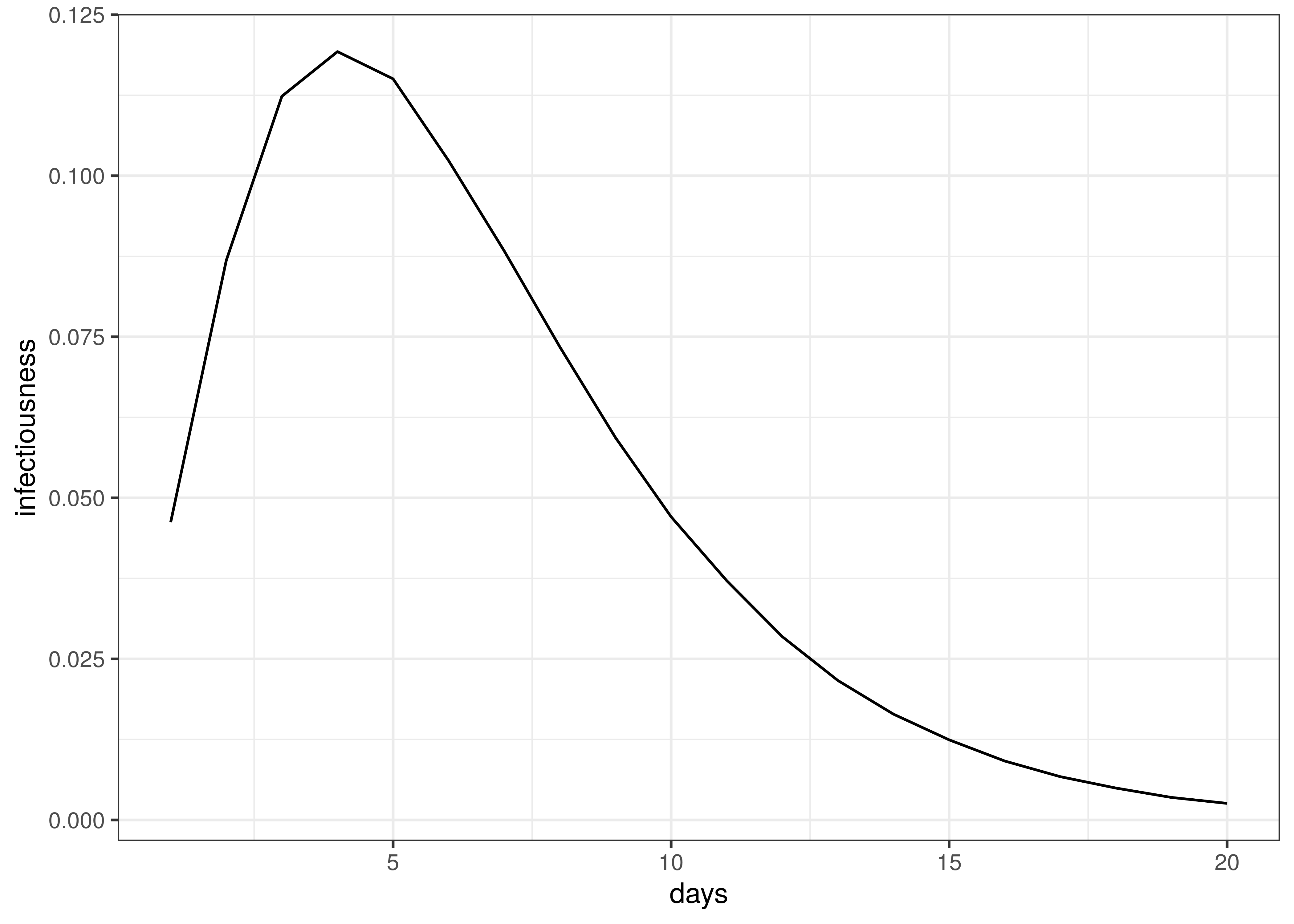
Infectiousness / Serial Interval
Time to death follows this distribution:
\(\pi \sim Gamma(5.1,0.86)+Gamma(17.8,0.45)\)
The distribution of time to death is plotted below.
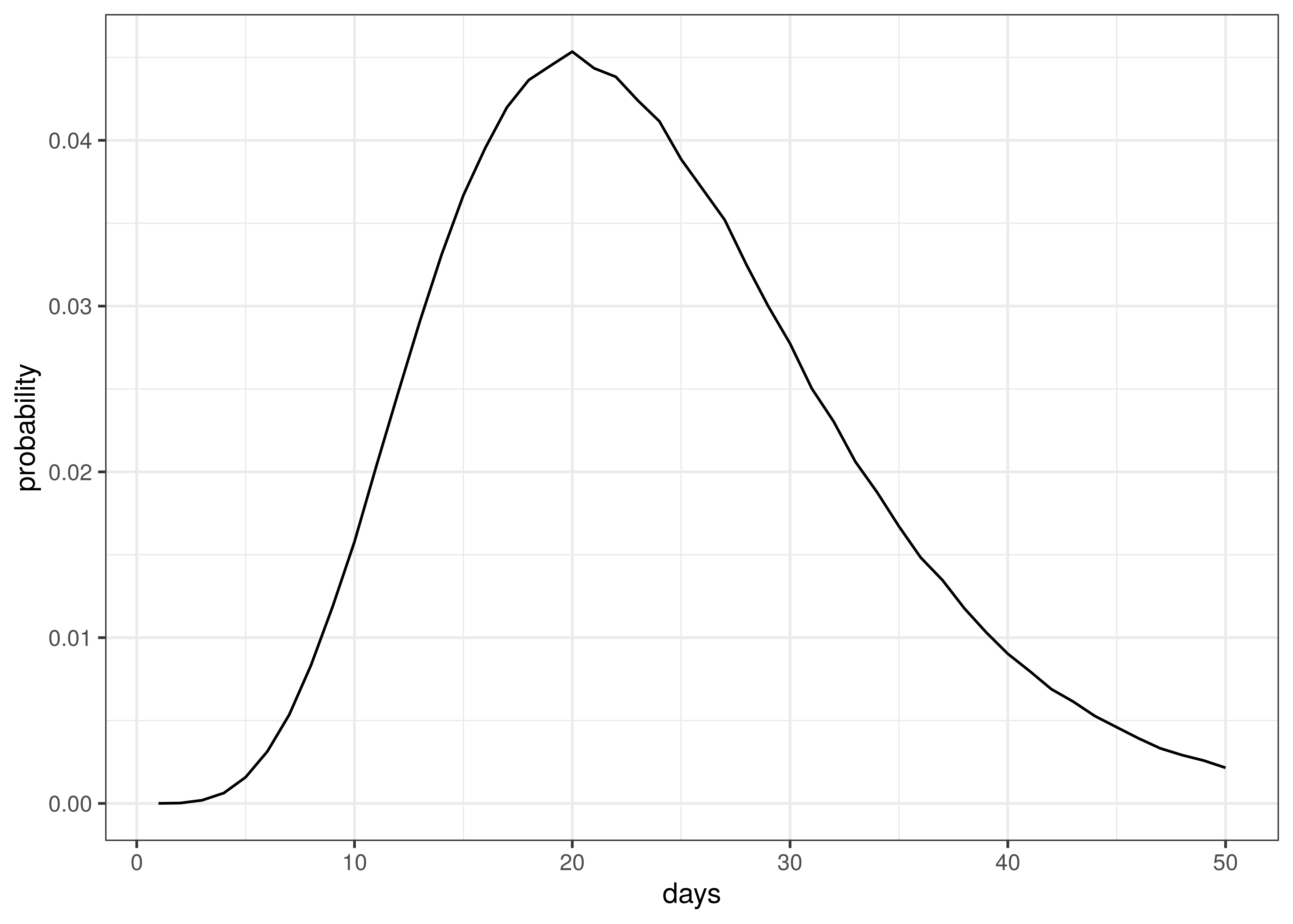
Distribution of Time to Death since Infection
The above implies an average time to death of 23 days.
A beta distribution is assumed for \(\psi_m\):
\(\psi_m \sim B(27,3)\)
The above distribution has a mean of 0.9, which is an assumption based on early indications that the majority of excess deaths are due to COVID-19. The distribution above implies that the probability \(\psi_m\) is below 0.8 is roughly 0.05. It is estimated that reported deaths in Western Cape is 70-80% of excess deaths, indicating a possible lower bound on the proportion of excess deaths that are due to COVID-19.
11.3 Death and Confirmed Case Data
Death and case data were used from [22]. This data set contains provincial case and death data as released by National Institute of Communicable Diseases (NICD). These data are shown for comparison purposes only as the model calibrates against excess deaths.
11.4 Excess Deaths
Excess deaths are taken from [4]. These excess deaths only contain deaths from 6 May 2020 and later (depending on when excess deaths were observed to start in each province). Reported COVID-19 deaths prior to these dates were included and treated as excess deaths.
Any negative excess deaths are set to zero.
Below weekly excess deaths for each province is plotted:
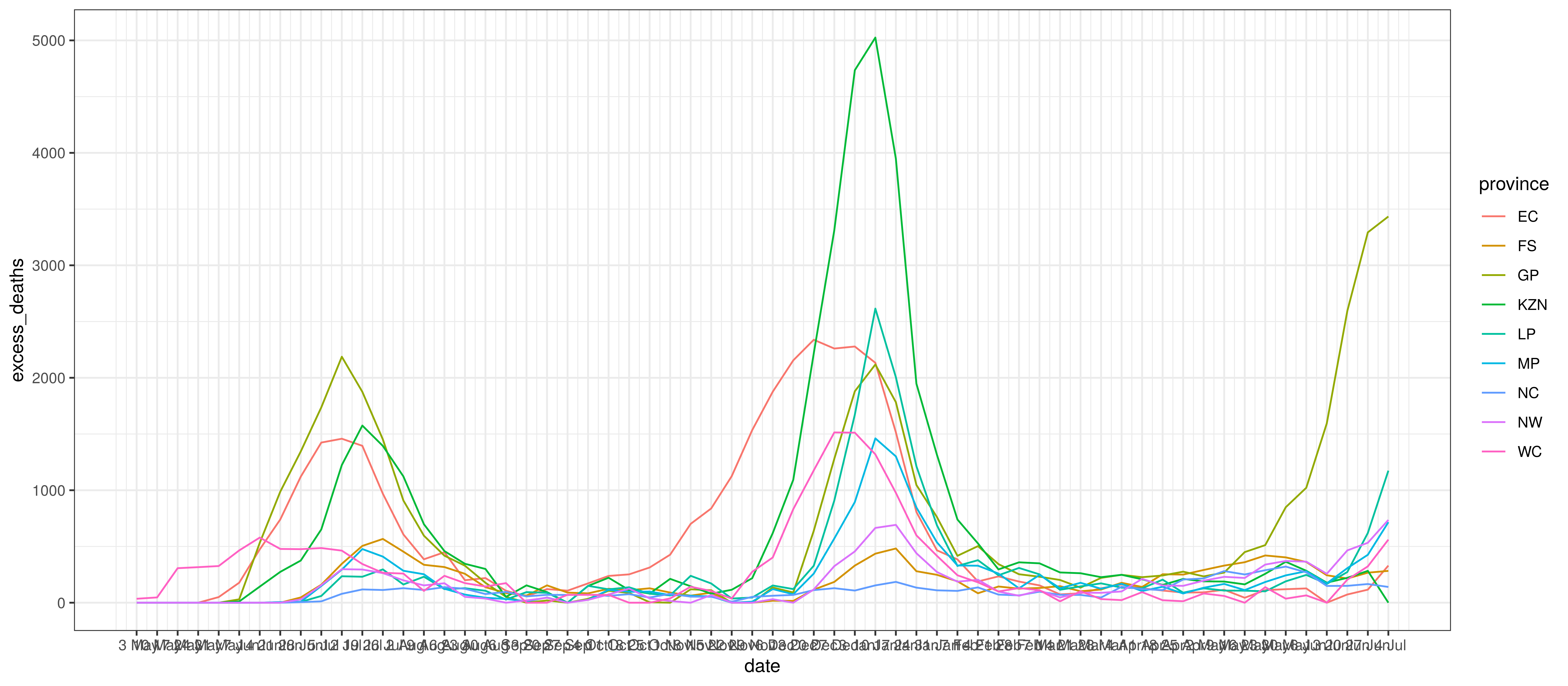
Excess Deaths by Province and Week
11.5 Infection Fatality Rates (IFR)
The age-specific infection attack rates (IAR) was was calculated using the output of the squire R package [13]. It produces age-specific infection attack rates (IAR). The projection was done using the default parameters for South Africa and the resultant attack rate (\(a_{x}\)) for each 5-year age band was obtained (\(x\)).
Per age infection fatality rates from [10] was used (\(ifr_{x}\)). These are slightly lower than those from [11], [12] and [13].
Additionally HIV prevalence by age-band and province, \(i_{x,m}^{HIV}\) was taken into account from [23] as well as results from [24]. In [24] it is shown that lives with HIV have higher COVID-19 mortality once infected. Based on these results it is assumed to be three times COVID-19 mortality below 55 and double mortality from age 55 upwards (\(m_x^{HIV}\)).
These \(a_{x}\) and \(ifr_{x}\) and HIV adjustments were then applied to the South African population per province and age band as per [25] and weighted IFRs calculated as follows.
\(ifr_{m}=\frac{\sum_{x}N_{x,m} \cdot a_{x} \cdot ifr_{x}( (1-i_{x,m}^{HIV}) +i_{x,m}^{HIV} \cdot m_x^{HIV})}{\sum_{x}N_{x,m}}\)
Here \(N_{x,m}\) is the population in a particular province (\(m\)) and age band (\(x\)).
Below the resultant \(ifr_{m}\) are tabulated:
| Province | IFR |
|---|---|
| EC | 0.64% |
| FS | 0.48% |
| GP | 0.36% |
| KZN | 0.41% |
| LP | 0.49% |
| MP | 0.41% |
| NC | 0.5% |
| NW | 0.43% |
| WC | 0.44% |
| South Africa | 0.44% |
The differences between provinces reflect the different age profiles in those provinces as per [25] and also differences in HIV prevalence. This seems low compared to the IFRs in [18], but may be reasonable given the younger profile of the South African population.
11.6 Mobility Indexes
Google has released aggregated mobility data for various countries and for sub-regions in those countries. These data are generated from devices that have enabled the Location History in Google Maps. This feature is available both on Android and iOS devices but is off by default.
For South Africa, these data contain the mobility indexes for each province. These are described in [5] as follows:
- Grocery & pharmacy: Mobility trends for places like grocery markets, food warehouses, farmers markets, specialty food shops, drug stores, and pharmacies.
- Parks: Mobility trends for places like local parks, national parks, public beaches, marinas, dog parks, plazas, and public gardens.
- Transit stations: Mobility trends for places like public transport hubs such as subway, bus, and train stations.
- Retail & recreation: Mobility trends for places like restaurants, cafés, shopping centres, theme parks, museums, libraries, and movie theatres.
- Residential: Mobility trends for places of residence.
- Workplaces: Mobility trends for places of work.
These measure changes in mobility relative to a baseline established before the epidemic. For example, -30% implies a 30% reduction in mobility from pre-COVID-19 mobility.
As per [7] these data were combined into an average mobility index for each province which was an average of all mobility indexes excluding:
- Residential
- Parks
In [1] three indexes were used (Residential, Transit and the rest). This was reduced for this paper due to limited data.
11.7 Variants
Below we plot the assumed proportion of infections due to the Beta variant, designated by \(I_{t}^{beta}\) and \(I_{t}^{delta}\) in the model above.
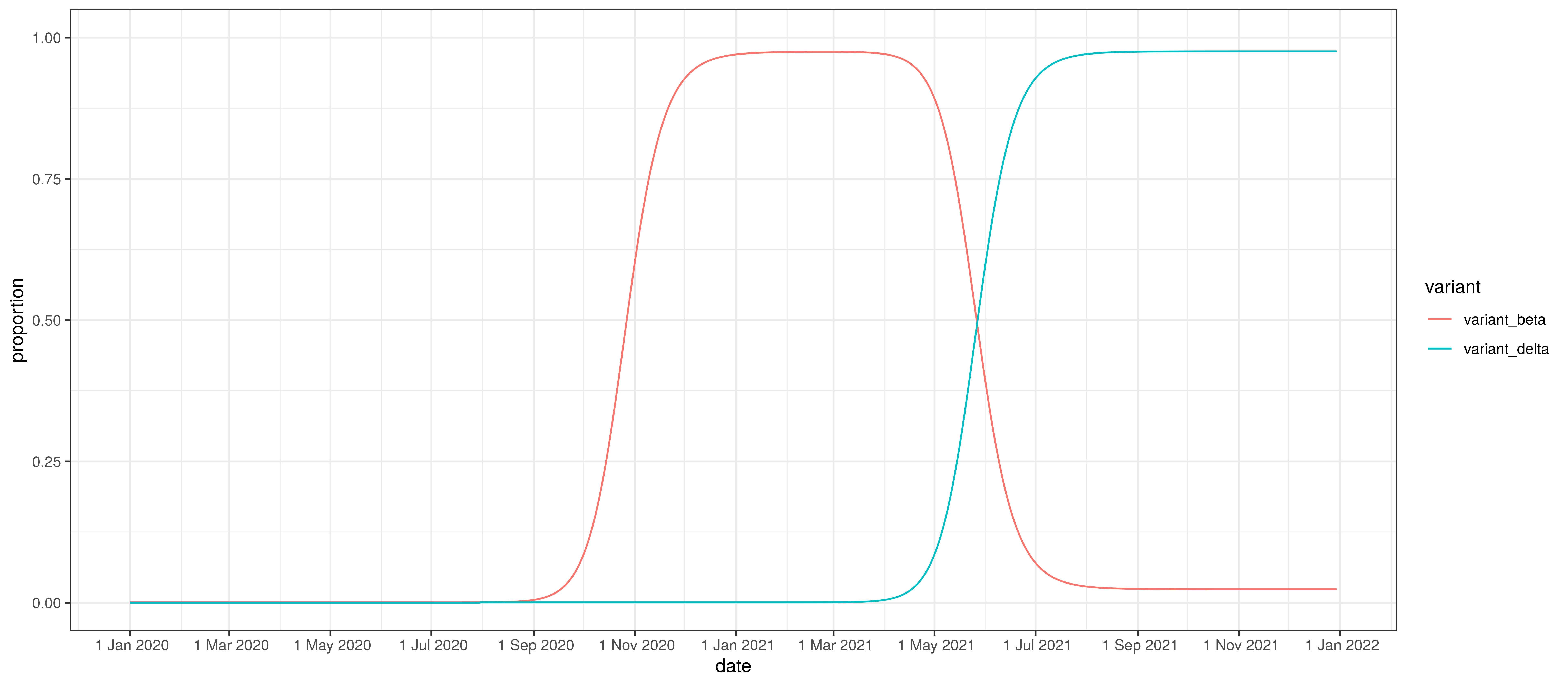
Proportion of infections by variant
12 Conclusion
This paper has set out to show how a Bayesian model can be fitted to the South African data. From the process it becomes clear that there remains significant uncertainty with all matters relating this epidemic. It is therefore likely that the model will not be accurate.
This paper has however attempted to allow for uncertainty using the Bayesian approach here which results in at least some distribution of possible results, some of which are definitely catastrophic and some of which are less severe.
It is hoped that this is a useful contribution to the ongoing research on the epidemic.